Historically, Dataflow Streaming Engine has offered exactly-once processing for streaming jobs. Recently, we launched at-least-once streaming mode as an alternative for lower latency and cost-of-streaming data ingestion. In this post, we will explain both streaming modes and provide guidance on how to choose the right mode for your streaming use case.
Exactly-once: what it is and why it matters
Applications that react to incoming events sometimes require that each event be reflected in the output exactly once — meaning the event is not lost, nor accepted more than a single time. But as the processing pipeline scales, load-balances, or encounters faults, that deduplication of events imposes a computational cost, affecting overall cost and latency of the system.
Dataflow Streaming provides an exactly-once guarantee, meaning that the effects of data processed in the pipeline are reflected at least and at most once. Let’s unpack that a little bit. For every arriving message, whether it’s from an external source or an upstream shuffle, Dataflow ensures that the message will be processed and not lost (at-least-once). Additionally, results of that processing that remain within the pipeline, like state updates and outputs to a subsequent shuffle to the next pipeline stage, are also reflected at-most once. This guarantee enables, among other things, performing exact aggregations, such as exact sums or counts.
Exactly-once inside the pipeline is usually only half the story. As pipeline authors and runners, we really want to get the results of processing out of Dataflow and into a downstream system. Here we run into a common roadblock: no general at-most-once guarantee is made about side-effects of the pipeline. Without further effort, any side-effect, such as output to an external store, may generate duplicates. Careful work must be done to orchestrate the writes in a way that avoids duplicates. The key challenge is that in the general case, it is not possible to implement exactly-once operation in a distributed system without a consensus protocol that involves all the actors. For internal state changes, such as state updates and shuffle, exactly-once is achieved by a careful protocol.With sufficient support from data sinks, we can thus have exactly-once all the way through the pipeline and to its output. An example is the storage write version of the BigQueryIO.Write implementation, which ensures exactly-once data extraction to BigQuery.
But even without exactly-once semantics at the sink, exactly-once semantics within the pipeline can be useful. Duplicates on the output may be acceptable, as long as they are duplicates of correct results — with exactly-once having been required to achieve this correctness.
At-least once: what it is and why it matters
There are other use cases where duplicates may be acceptable, for example ETL or Map-Only pipelines that are not performing any aggregation but rather only per-message operations. In these cases, duplicates are simple replays of data through the pipeline.
But why wouldn’t you choose to use exactly-once semantics? Aren’t stronger guarantees always better? The reason is that achieving exactly-once adds to pipeline latency and cost. This happens for several reasons, some obvious, and some quite subtle. Let’s take a deeper look.
In order to achieve exactly-once, we must store and read exactly-once metadata. In practice, the storage and read costs incurred to do this turn out to be quite expensive, especially in pipelines that otherwise perform very little I/O. Less intuitively, having to perform this metadata-based deduplication dictates how we implement the backend.
For example, in order to deduplicate messages across the shuffle we must ensure that all replays are idempotent — which means we must checkpoint the results of processing before they are sent to shuffle — which again increases cost and latency.
Another example: to de-duplicate the input from Pub/Sub, we must first re-shuffle incoming messages on keys that are deterministically derived from a given message because the deduplication metadata is stored in the per-key state. Performing this shuffle using deterministic keys exposes us to additional cost and latency. In the next section we lay out the reasons for this in more detail.
We cannot assume that at-least-once semantics are acceptable for the user, so we default to the strictest, semantics, i.e., exactly-once. If we know beforehand that at-least-once processing is acceptable, and we can relax our constraints, then we can make more cost- and latency-beneficial implementation decisions.
Exactly-once vs. at-least-once when reading from Pub/Sub
Pub/Sub reads’ latency and cost in particular benefit from at-least-once mode. To understand why, let’s look closer at how exactly-once deduplication is implemented.
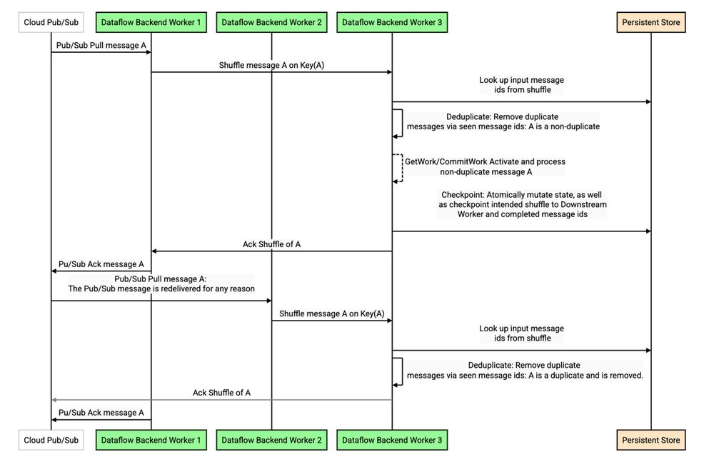
Pub/Sub reads are implemented in the Dataflow backend workers. To acquire new messages, each Dataflow backend worker makes remote procedure calls (RPCs) internally to the Pub/Sub service. Since RPCs can fail, workers may crash, or other sources of failure are possible, and messages will be replayed until successful processing is acknowledged by the backend worker. Pub/Sub and backend workers are dynamic systems, without static partitioning, meaning that replays of messages from Pub/Sub are not guaranteed to arrive at the same backend worker. This poses a challenge when deduplicating these messages.
In order to perform deduplication, the backend worker puts these messages through a shuffle, attaching a key internally to each message. The key is chosen deterministically based on the message, or a message id attribute if configured1, so that a replay of a duplicate message is deterministically shuffled to the same key. Doing so allows deduplicating replays from Pub/Sub in the same manner that shuffle replays are deduplicated between stages in the Dataflow pipeline (see this detailed discussion), as illustrated in the sequence diagram below:
This design contributes to cost and latency in two significant ways. First, as with all deduplication in the Dataflow backend, a read against the persistent store may be required. While heavily optimized with caches and bloom filters, it cannot be completely eliminated. Second, and often even more significant, is the need to shuffle the data on a deterministic key. If a particular key or worker is slow or becomes a bottleneck, this creates head-of-line blocking that prevents other traffic from flowing — an artificial constraint since the messages in the queue are not semantically tied to this key.
When at-least-once processing is acceptable, we can both eliminate the cost associated with reads from the persistent store and the shuffling of messages on a deterministic key. In fact, we can do better — we still shuffle the messages, but the key we pick instead is the current “least-loaded” key, meaning the key that is currently experiencing the least queueing. In this way, we evenly distribute the incoming traffic to maximize throughput, even when some keys or workers are experiencing slowness.
We can see this in action in a benchmark where we simulate stragglers, e.g., slow writes to an external sink, by artificially delaying arbitrary messages at low probability for multi-minute intervals.
Compare the throughput of the exactly-once pipeline on the left to the throughput of the at-least-once pipeline on the right. The at-least-once pipeline can sustain much more consistent throughput in the presence of such stragglers, dramatically decreasing average latency. In other words, even though both cases still have high tail latency, the latency outliers no longer affect the bulk of the distribution in the at-least-once configuration.
Benchmarks: at-least-once vs. exactly-once
Here are three representative benchmark streaming jobs to evaluate the impact of streaming-mode choice on costs. To maximize the cost benefit, we enabled resource-based billing and aligned I/O to the streaming mode. Here is what we observed:
Note that cost depends on multiple factors such as data-load characteristics, the specific pipeline composition, configuration and the I/O used. Therefore, our benchmarking results may differ from what you observe in your test and production pipelines.
Spotify’s own testing supported the Dataflow team’s findings:
“By incorporating at-least-once mode in our platform that is built on Dataflow, Pub/Sub, and Bigtable, we have seen a portion of our Dataflow jobs cut costs by 50%. Since this is used by several consumers, 7 downstream systems are now cheaper overall with this simple change. Because of the way this system works, there has been 0 effects of duplicates! We plan on turning this feature on in more jobs that are compatible to cut down our Dataflow costs even more.” –Sahith Nallapareddy, Software Engineer, Spotify
Choose the right streaming mode for your job
When creating streaming pipelines, choosing the right mode is essential. The critical factor is to determine whether the pipeline can tolerate duplicate records in the output or any intermediate processing stages.
At-least-once mode can help optimize cost and performance in the following cases:
Map-only pipelines performing idempotent per-message operations, e.g. ETL jobs
When deduplication happens in the destination, e.g., in BigQuery or Bigtable
Exactly-once mode is preferable in the following cases:
Use cases that cannot tolerate duplicates within Dataflow
Pipelines that perform exact aggregations as part of stream processing
Map-only jobs that perform non-idempotent per-message operations
At-least-once streaming mode is now generally available for Dataflow streaming customers. You can enable at-least-once mode by setting the at-least-once Dataflow service option when starting a new streaming job using the API or gcloud. To get started, we also offer a selection of commonly used Dataflow streaming templates that support the streaming modes.
Editor’s note: The post is part of a series showcasing partner solutions that are Built with BigQuery.
Data is paramount when making critical business decisions. Whether it’s identifying new opportunities, streamlining operations, or delivering more value to customers, leadership wants to know that they have the facts on their side when making crucial choices about the future. That means having and evaluating the right data – the data that comes from their products.
Pendo provides companies with the most effective way to infuse product data into their greater business strategy. As a company on a mission to elevate the world’s experience with software, Pendo has created Data Sync, a product that makes it easier to connect valuable behavioral insights from applications to the broader business. With Data Sync, teams have visibility into data about customer engagement and health, regardless of where it sits in an organization.
Siloed product data is wasted product data
Without the ability to incorporate product-level behavioral insights into business reporting, companies can’t understand the holistic journey of their users. Given the current macroeconomic conditions, businesses are under extra pressure to retain and grow their existing customer base, and not understanding user behavior in its full context is a clear disadvantage.
Too often an incomplete picture of product usage is the result of compiling data together piece by piece or via an API pull, which doesn’t provide the value businesses need. This approach can distract and pull resources away from building a scalable, supported data strategy model. Without a single source of truth into product data, each team is left making crucial business decisions with only part of the picture. This results in siloed data and wasted insights that could help answer crucial questions, such as:
Are users deriving value from key product areas that align with commercial models?
Are customer cohorts as engaged and healthy as their point of renewal approaches?
When looking to maximize the lifetime value of customer accounts, what behavior trends can inform sales strategy?
Do customer teams have the insights they need to proactively address risk and churn?
Rich insights to answer crucial questions
There’s an alternative to this fragmented approach. With Pendo Data Sync for Google Cloud, teams can quickly make Pendo data available whenever they need it in Cloud Storage and access it in BigQuery, or any other data lake or warehouse. By connecting behavioral data from product applications (i.e., user interactions with them) with other key business data sources, Pendo enables organizations to make important decisions with confidence.
Pendo makes it easy to:
Easily access all historical behavioral and product utilization data. Structure and take action on the valuable data across your entire data ecosystem. In Google Cloud, data teams can maximize the value of BigQuery and Looker by integrating these additional datasets to help generate business insights that were previously unavailable.
Democratize data to drive informed decision making. Instantly join product data with the full breadth of all your key business data at the depth required to support a modern data-driven organization.
Drive better resource utilization. Remove the need to manually pull siloed data sets and give your data and engineering teams back time to spend on more valuable activities.
Get maximum ROI on your product insights. Enable every department — all the way up to the C-suite — to speak the same universal language of the business.
Make faster, more confident decisions. Put product data at the center of your decision-making processes.
Democratizing data to buttress the business
Pendo data acts as our customers’ primary source of truth for the applications they build, sell, and deploy. With Data Sync, these insights are no longer confined to the product teams using Pendo directly — they become available for all. With a straightforward extract, transform, and load (ETL) process, every department and cross-functional initiative can easily access Pendo data in a centralized location.
To date, Data Sync customers have used Pendo data for a wide variety of use cases. These include measuring the impact of product improvements on sales and renewals, identifying friction in your end-to-end user journey, and calculating a comprehensive customer health score across all data sources to shape renewal strategy. Other teams have also leveraged Pendo data to create a churn-risk model based on a foundation of product usage and sentiment signals or identify up-sell and cross-sell opportunities to drive data-informed account growth.
Pendo Data Sync is ‘Built with BigQuery’
Building Data Sync on top of Google Cloud made the development and initial rollout of the solution very straightforward. Pendo’s engineering team was able to leverage its existing knowledge of Google Cloud products and services to build the beta version of Data Sync. This version was then rolled out to design partners using Google Cloud, helping to standardize the methods and best practices for pulling bulk Pendo data from Cloud Storage into BigQuery. Additionally, Pendo’s data science team uses BigQuery as its data warehouse solution and Looker as its primary business intelligence tool. The data team became the first “alpha” customer for Data Sync, partnering with engineering to design the product’s data structure, ETL best practices, and help documentation.
Looking ahead, Pendo is exploring even deeper integration into Google Cloud, including data sharing directly in Analytics Hub.
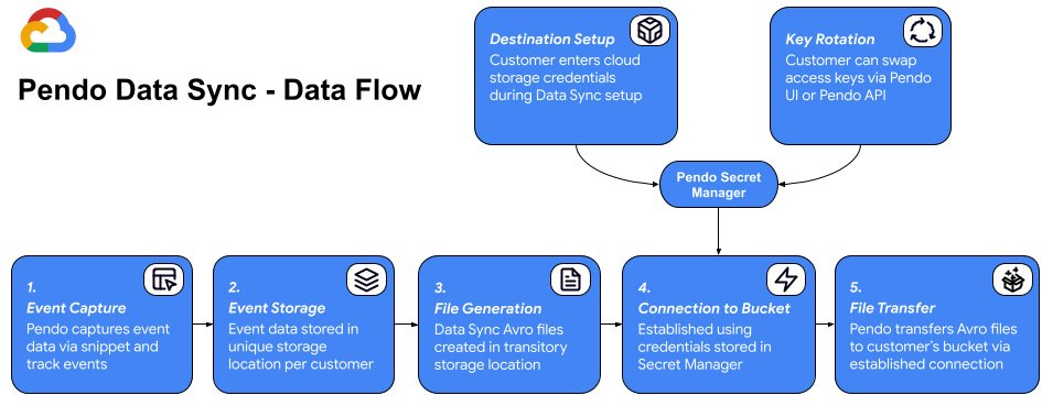
Below is a diagram of the architecture Data Sync uses for its data flow:
Utilize your product data to the fullest
By partnering with Pendo, you can take maximum advantage of your product utilization data. Combining quantitative and qualitative feedback with other related data sets can give you a holistic view into user engagement and health, empowering your teams to make strategic decisions about customer retention and growth — backed by data.
You can also request a custom demo with a Pendo team member to learn how your business can use Pendo to increase customer engagement and health.
The ‘Built with BigQuery’ advantage for ISVs and data providers
Built with BigQuery helps companies like Pendo build innovative applications with Google Data Cloud. Participating companies can:
Accelerate product design and architecture through access to designated experts who can provide insight into key use cases, architectural patterns, and best practices.
Amplify success with joint marketing programs to drive awareness, generate demand, and increase adoption.
BigQuery gives ISVs the advantage of a powerful, highly scalable unified AI lakehouse that’s integrated with Google Cloud’s open, secure, sustainable platform. To find how to harness the full potential of your data to drive innovation, learn more about Built with BigQuery
We are excited to invite customers to join a preview of new SQL features that simplify time series analysis in BigQuery. These new features simplify writing queries that perform two of the most common time series operations: windowing and gap filling. We are also introducing the RANGE data type and supporting functions. The RANGE type represents a continuous window of time and is useful for recording time-based state of a value. Combined, these features make it easier to write time series queries over your data in BigQuery.
Time-series analytics and data warehouses
Time-series data is an important, and growing class of data for many enterprises. Operational data like debug logs, metrics, and event logs are inherently time-oriented and full of valuable information. Additionally, connected devices common in manufacturing, scientific research, and other domains continually produce important metrics that need to be analyzed. All of this data follows the same pattern: the data is reported as values at a specific time, and deriving meaning from that data requires understanding how it changes over time.
Users with time-series analytics problems have traditionally relied on domain-specific solutions that result in harder to access data silos. Additionally, they often have their own query languages, which require additional expertise to use. Organizations looking to analyze their time-series data alongside the rest of their data must invest in pipelines that first clean and normalize the data in one store before exporting it to their data warehouse. This slows down time-to-insights and potentially hides data from the users who could build value from the data. Adding more time-series analytics features to BigQuery SQL democratizes access to this valuable data. Organizations can now leverage BigQuery’s scalable serverless architecture to store and analyze their time-series data alongside the rest of their business data without having to build and maintain expensive pipelines first.
Introducing time-series windowing and gap filling functions
The first step in most time-series queries is to map individual data points to output windows of a specific time duration and alignment. For example, you want to know the average of a sampled value every ten minutes over the past twelve hours. The underlying data is often sampled at arbitrary times so the user’s query must include logic to map the input times to the output time windows. BigQuery’s new time bucketing functions provide a full-featured method for performing this mapping.
Let’s look at an example using a time series data set showing the air quality index (AQI) and temperature recorded over part of the day. Each row in the table represents a single sample of time-series data. In this case, we have a single time series for the zip code 60606, but the table can easily hold data for multiple time series, all represented by their zip code.
Before doing additional processing we’d like to assign each row to a specific time bucket that is two-hours wide. We’ll also aggregate within those windows to compute the average AQI and maximum temperature.
code_block
<ListValue: [StructValue([(‘code’, ‘SELECTrn TIMESTAMP_BUCKET(time, INTERVAL 2 HOUR) AS time,rn zip_code,rn CAST(AVG(aqi) AS INT64) AS aqi,rn MAX(temperature) AS max_temperaturernFROM mydataset.environmental_data_hourlyrnGROUP BY zip_code, timernORDER BY zip_code, time;rnrn+———————+———-+—–+—————–+rn| time | zip_code | aqi | max_temperature |rn+———————+———-+—–+—————–+rn| 2020-09-08 00:00:00 | 60606 | 23 | 66 |rn| 2020-09-08 02:00:00 | 60606 | 22 | 60 |rn| 2020-09-08 06:00:00 | 60606 | 25 | 56 |rn+———————+———-+—–+—————–+’), (‘language’, ”), (‘caption’, <wagtail.rich_text.RichText object at 0x3e2b0ac92460>)])]>
Note that we can use any valid INTERVAL to define the width of the output window. We can also define an arbitrary origin for aligning the windows if we want to start the windows at something other than 00:00:00.
Gap filling is another common step in time-series analysis that addresses gaps in time of the underlying data. A server producing metrics may reset, stopping the flow of data in the progress. A lack of user traffic may mean gaps in event data. Or, data may be inherently sparse. Users want to control how these gaps are filled in before joining with other data or preparing it for graphing. The newly released GAP_FILL table valued function does just that.
In our previous example, we have a gap between 02:00 and 06:00 in the output data because there is no raw data between 04:00:00 and 05:59:59. We would like to fill in that gap before joining this data with other time-series data. Below, we demonstrate two modes of backfill supported by the GAP_FILL TVF: “last observation carried forward” (locf) and linear interpolation. The TVF also supports inserting nulls.
code_block
<ListValue: [StructValue([(‘code’, “WITH aggregated_2_hr AS (rn SELECTrn TIMESTAMP_BUCKET(time, INTERVAL 2 HOUR) AS time,rn zip_code,rn CAST(AVG(aqi) AS INT64) AS aqi,rn MAX(temperature) AS max_temperaturern FROM mydataset.environmental_data_hourlyrn GROUP BY zip_code, timern ORDER BY zip_code, time)rnrnSELECT *rnFROM GAP_FILL(rn TABLE aggregated_2_hr,rn ts_column => ‘time’,rn bucket_width => INTERVAL 2 HOUR,rn partitioning_columns => [‘zip_code’],rn value_columns => [rn (‘aqi’, ‘locf’),rn (‘max_temperature’, ‘linear’)rn ]rn)rnORDER BY zip_code, time;rnrnrn+———————+———-+—–+—————–+rn| time | zip_code | aqi | max_temperature |rn+———————+———-+—–+—————–+rn| 2020-09-08 00:00:00 | 60606 | 23 | 66 |rn| 2020-09-08 02:00:00 | 60606 | 22 | 60 |rn| 2020-09-08 04:00:00 | 60606 | 22 | 58 |rn| 2020-09-08 06:00:00 | 60606 | 25 | 56 |rn+———————+———-+—–+—————–+”), (‘language’, ”), (‘caption’, <wagtail.rich_text.RichText object at 0x3e2b0ac92d60>)])]>
GAP_FILL can also be used to produce aligned output data without having to bucket the input data first.
Combined, these new bucketing and gap-filling operations provide key building blocks of time-series analytics. Users can now leverage BigQuery’s serverless architecture, high-throughput streaming ingestion, massive parallelism, and built-in AI to derive valuable insights from their time-series data alongside the rest of their business data, all without relying on a separate data silo.
Importantly, these new functions align with the standard SQL syntax and semantics analytics that experts are familiar with. There is no need to learn a new language or a new computation model. Simply add these functions into your existing workflows and start delivering insights.
Introducing the RANGE data type
The RANGE type and functions make it easier to work with contiguous windows of data. For example, RANGE<DATE> “[2024-01-01, 2024-02-01)” represents all DATE values starting from 2024-01-01 up to and excluding 2024-02-01. RANGE can also be unbounded on either end, representing the beginning and end of time respectively. RANGE is useful for representing a state that is true, or valid, over a contiguous period of time. Quota assigned to a user, the exchange rate of a currency over different times, the value of a system setting, or the version number of an algorithm are all great examples.
We are also introducing features that allow you to combine or expand RANGEs at query time. RANGE_SESSIONIZE is a TVF that allows you to combine overlapping or adjacent RANGEs into a single row. The table below shows how users can use this feature to create a smaller table with the same information:
RANGE_SESSIONIZE finds all overlapping ranges and outputs the session range, which is a union of all the ranges that overlap within the (sensor_id, flow) partition. We finally group by the session ranges to output a table that combines the overlapping ranges:
You can do much more with RANGE. For example, you can use RANGE to JOIN a timestamp table with a RANGE table or emulate the behavior of an AS OF JOIN. See more examples in the RANGE and time series documentation.
Getting started
To use the new time series analysis features, all you need is a regular table with some time series data in it. You can even try experimenting with one of the existing public datasets. Check out the documentation to learn more and get started. Give these new features a try and let us know if you have feedback.
One of the challenges organizations face today is harnessing the potential of their collected data. To do so, you need to invest in powerful data platforms that can efficiently manage, control, and coordinate complex data flows and access across various business domains.
RealTruck, a leader in aftermarket accessories for trucks and off-road vehicles, stands out for its omnichannel approach, which successfully integrates over 12,000 dealers and a robust online presence at RealTruck.com. Operating from 47 locations across North America, the company initially faced significant data challenges due to its extensive offline network and diverse customer touchpoints. To address these complexities, the data team at RealTruck decided to develop a data platform that could serve as a source of truth for executives and every manager in the organization, providing data to support business decision-making. The goal was to gain visibility into and control over all collected assets, monitor data flows, manage costs, and ensure the high reliability of the data platform.
RealTruck’s data team chose BigQuery as the center element of their data platform for its high security standards, scalability, and ease of use. As a serverless data platform, BigQuery allows the team to focus on strategic analysis and insights rather than on managing infrastructure, thereby enhancing their efficiency in handling large volumes of data.
RealTruck data is gathered from various sources, including manufacturers, dealers, marketing campaigns, web and app customer interactions, and sales transactions. This data, along with the company’s data pipelines, vary in format, structure, and cadence. The diversity and number of external data sources present significant maintenance challenges and operational complexity.
RealTruck also added Masthead Data, a Google Cloud Ready partner for BigQuery, to help its data team identify any pipeline or data issues that affect business users or data consumers. When selecting a partner to integrate with BigQuery, RealTruck needed the ability to monitor for errors in other solutions used to build its data platform, which could result in downtime. This included Cloud Storage, BigQuery Data Transfer Service, Dataform, and other Google Cloud services.
Together, BigQuery and Masthead enabled RealTruck’s data team to deliver on two of its biggest commitments — ensuring the accuracy of the company’s data and resolving any doubts about the performance of data pipelines.
Mastering data platform complexity: Visibility, cost efficiency, and anomaly detection
As RealTruck began building out its data platform with BigQuery, the data team realized that there were still some issues around complexity that needed to be solved.
Limited visibility of pipeline performance: Ingesting data into the platfrom from numerous sources using various solutions made it difficult to track pipeline failures or data system errors. This limitation hindered RealTruck’s ability to maintain reliable data. Cost control: BigQuery enabled the data team to develop a decentralized data platform, boosting agility to create data pipelines and assets. However, this approach requires more refined management of resources to ensure cost-effectiveness, given the scalable processing power. To sustain efficiency, the team sought granular visibility into every process and its associated costs. Anomaly detection across the data platform: Tables in BigQuery are regularly used as sources for data products, requiring vigilant monitoring for issues like freshness, volume spikes, or missing values. The ability to automatically identify outliers or unexpected behavior is key for building trust in the data platform among business users.
Masthead and BigQuery: Achieving data platform reliability for RealTruck
To overcome these challenges, RealTruck implemented Masthead Data to enhance the reliability of BigQuery data pipelines and assets in its data platform.
Masthead provided visibility into potential syntax errors and system issues caused by using various ingestion tools. Automating observability enabled RealTruck to detect pipeline or data environment issues in real time, allowing the team to address them before they impacted downstream data products or platform users.
For example, Masthead provided real-time alerts and robust column-level lineage and data dictionary features to help troubleshoot downtime in the data platform within minutes. As a result, the RealTruck data team was able to trace an error or anomaly and assess the full impact of it on pipelines or BigQuery tables. Column-level lineage also made it easier for the team to respond quickly and collaborate more effectively when resolving issues.
In addition, Masthead’s unique approach of using logs to monitor time-series tables for freshness, volume, and schema changes allowed RealTruck to have an overarching view of the health of all its BigQuery tables without increasing compute costs. Masthead also integrates with Google Dataplex, enabling the RealTruck team to implement rule-based data quality checks to catch any anomalies in metrics.
RealTruck also leveraged Masthead’s Compute Cost Insights for BigQuery to gain granular visibility into BigQuery storage and pipeline costs as well as any third-party solutions used in the data platform. These features have helped the data team identify and cleanup orphan processes and expired assets, making the costs of the data platform more manageable and transparent.
“One of the main reasons RealTruck chose Masthead was its unique architecture, which does not access our data. This was a critical factor in our decision, especially given our ambitious global growth plans and the increasingly complex data privacy regulations worldwide. Masthead, as a Google Cloud Partner, complimentary to Google Cloud BigQuery, is compliant with data privacy and security regulations at the architectural level, ensuring that our data remains secure,aligning perfectly with our strategic objectives.
The ability to achieve comprehensive observability of all our BigQuery data pipelines and tables through a no-code integration, which was set up in just 15 minutes and began delivering value within a few hours, has been transformative. It has enabled the RealTruck team to gain valuable insights into pipeline costs and data flows swiftly across our entire data platform, reinforcing the reliability and strategic value of our data-driven initiatives.” – Chris Wall, Director of BI & Analytics, RealTruck
Google Cloud has become the backbone of RealTruck’s data infrastructure, providing efficient data governance and management with minimum configuration required. BigQuery offers Google Cloud’s world-class default encryption and sophisticated user access management features, which allows RealTruck to distribute, store, and process its data with confidence, knowing its data is secure.
Masthead’s approach to processing logs and metadata also aligns well with Google Cloud’s approach to security and privacy, offering a single view of pipeline and data health across RealTruck’s entire data environment. This consolidated view has enabled the data team to shift from ad-hoc solutions to making strategic improvements to the data platform. This enhanced perspective has been vital for building a data platform that business users trust, allowing RealTruck to efficiently tackle data errors and manage costs. The efficient use of BigQuery in combination with Masthead significantly reduced the risk of unnoticed issues impacting business operations, reinforcing the importance of data in decision-making.
At Palo Alto Networks, our mission is to enable secure digital transformation for all. Part of our growth through mergers and acquisitions has led to a large, decentralized structure with many engineering teams that contribute to our world-renowned products. Our teams have more than 170,000 projects on Google Cloud, each with its own resource hierarchy and naming convention.
Our Cloud Center of Excellence team oversees the organization’s central cloud operations. We took over this complex brownfield landscape that has been growing exponentially, and it’s our job to make sure the growth is cost-effective, follows cloud hygiene, and is secure while still empowering all Palo Alto Networks product engineering teams to do their best work.
However, it was challenging to identify which project belonged to which team, cost center, and environment, which is a crucial starting point for our team’s work. We overtook a large automated labeling effort three years ago, which got us to over 95% coverage on tagging for team, owner, cost center and environment. However the last 5% turned out to be more difficult. That’s when we decided we could use machine learning to make our lives easier and our operations more efficient. This is the story of how we achieved that with BigQuery ML, BigQuery’s built-in machine learning feature.
Reducing ML prototyping turnaround from two weeks to two hours
Identifying the owner, environment, and cost center for each cloud project was challenging because of the sheer number of projects and their various naming conventions. We often found mislabeled projects that were assigned to incorrect teams or to no team at all. This made it difficult to determine how much teams were spending on cloud resources.
To correctly assign team owners on dashboards and reports, a finance team member had to sort hundreds of projects by hand and contact possible owners, a process taking weeks. If our investigation was inconclusive, the projects were marked as ‘undecided.’ As this list grew, we only looked into high-cost projects, leaving low-spend projects without a correct ownership label.
When questions regarding project ownership surfaced, our team looked for keywords in a project’s name or path which gave us clues about which team was connected to it. But we followed our intuition based on keywords, and we knew that we could use machine learning to do the same. It was time to automate this manual process.
Initially we used Scikit-learn for machine learning and Python libraries to write the code from scratch, and it took almost two weeks to build a working model to help us start training end-to-end prediction algorithms. While we got good results, it was a small-scale prototype that couldn’t handle the volumes of data we needed to ingest.
Palo Alto Networks already used BigQuery extensively, making it easy to access our data for this project. The Google Cloud team suggested we instead try BigQuery ML to prototype our project and it just made sense. With BigQuery ML, prototyping the entire project took a couple of hours. We were up and running within the same afternoon, with 99.9% accuracy. We tested it on hundreds of projects and got correct label predictions every time.
Boosting developer productivity while democratizing AI
Immediately after deploying BigQuery ML, we could use and test a variety of models that were readily available from its library to see what worked best for our project, eventually landing on the boosted trees model. Previously, using Python Scikit-learn, training different algorithms for testing took up to three hours each time we found that they weren’t accurate enough. With BigQuery ML, that trial-and-error loop is much shorter. We simply replace the keyword and do one hour of training to try a new model.
Similarly, the developer time required for this project has reduced significantly. In our previous iteration, we had more than 300 lines of Python code. We’ve now turned that into 10 lines of SQL in BigQuery, which is much easier to read, understand, and manage.
This brings me to AI democratization. We initially assigned this prototype to an experienced colleague because a project like this used to require an in-depth machine learning and Python background. Reading 300 lines of ML Python code would take a while and explaining it would take even longer, so no one else on our team could have done this manually.
But with BigQuery ML, we can look at the code sequence and explain it in five minutes. Anyone on our team can understand and modify it by knowing just a little about what each algorithm does in theory. BigQuery ML makes this work much more accessible, even for people without years of machine learning training.
Solving for greater visibility with 99.9% accuracy
This label prediction project now supports the backend infrastructure for all cloud operations teams at Palo Alto Networks. It helps to identify which team each project belongs to and sorts mislabeled projects, giving financial teams visibility into cloud costs. Our new labeling system gives us accurate, reliable information about our cloud projects with minimal manual intervention.
For now, this solution can tell us with 99.9% accuracy which team any given project belongs to, in which cost center, and in which environment. This feels like a gateway introduction. Now that we’ve seen the usefulness of BigQuery ML, and how quickly it can make things happen, we’ve been talking about how to extend its benefits to more teams and use cases.
For example, we want to implement this model as a service for financial operations and information security teams who may need more information about any project. If there’s a breach or suspicious activity for a project that isn’t already mapped, they could quickly use our model to find out who the affected project belongs to. We have mapping for 95-98% of our projects, but that last bit of unknown territory is the most dangerous. If something happens in a place where no one knows who’s responsible, how can it be fixed? Ultimately, that’s what BigQuery ML will help us solve.
Excited for what’s ahead with generative AI
One other project we’re excited about combines BigQuery with generative AI to empower non-technical users to get business questions answered using natural language. We’re creating a financial operations companion that understands who employees are, what team they belong to, what projects that team owns, and what cloud resources it is using, to provide all the relevant cost, asset, and optimization information from our Data Lake stored in BigQuery.
Previously, searching for this kind of information would require knowing where and how to write a query in BigQuery. Now, anyone who isn’t familiar with SQL, from a director to an intern, can ask questions in plain English and get an appropriate answer. Generative AI democratizes access to information by using a natural language prompt to write queries and combine data from multiple BigQuery tables to surface a contextualized answer. Our alpha version for this project is out and already showing good results. We look forward to building this into all of our financial operations tools.
Over the last two decades, cloud-based data management and analytics solutions have become more cost effective and flexible than their on-premises counterparts. But even among cloud providers there are differences in cost, flexibility, scalability, and AI readiness that impact a business’s bottom line. Choosing the right enterprise data warehouse (EDW) solution requires designing an effective data cloud strategy and understanding the underlying technology, operational capabilities, and pricing models of potential providers.
TechTarget’s Enterprise Strategy Group (ESG) did an extensive study to compare the quantitative and qualitative benefits that organizations can realize with Google Cloud BigQuery when compared with alternative solutions. Download the full report here.
Let’s look at some of the report’s key findings:
How to choose the right cloud-based enterprise data warehouse
Finding ways to decrease time to insights is only one step of selecting the right EDW. Teams also should consider total cost of ownership and potential upfront costs, the solution’s ability to efficiently scale up and down based on demand, and continuous innovation to support predictive AI, machine learning, and generative AI projects.
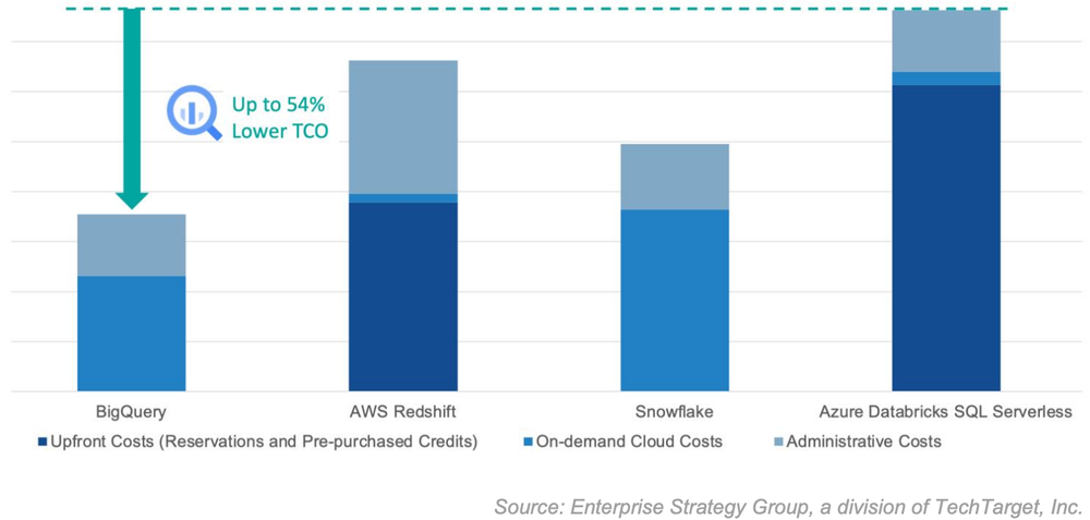
Across these three categories, ESG found that BigQuery eliminated upfront investment and planning requirements, reduced operational costs, and improved business agility. In fact, BigQuery customers save up to 54% in total cost of ownership compared to alternative cloud EDW offerings.
Here are some of the key reasons these factors play an outsized role in how and why businesses select their data and analytics platform.
High-performance EDW doesn’t have to break the bank
Investing in an EDW solution is a strategic choice with long-term consequences for data processing. That doesn’t mean it has to be an overwhelming financial decision. BigQuery doesn’t require any upfront investment to save on computing resources. Some providers analyzed in the study require an upfront purchase while others only offer their most competitive pricing to customers who commit to a large upfront purchase.
Signing on for a specific contract period means teams have to plan and size their configurations ahead of purchasing, as if they were on-premise nodes, or roughly estimate future node cluster and virtual data warehouse usage. BigQuery is fully managed and autoscales to a maximum number of predefined slots as needed, then returns to defined base levels when not in use, so organizations don’t need to commit to precalculated configurations. This can reduce compute usage by 30% to 40%.
Reducing operational costs while making data work harder
Transitioning to the cloud already helps to save on costs by eliminating management and maintenance of on-premise hardware. By selecting an EDW that’s fully managed and doesn’t require dedicated capacity monitoring, teams can easily manage data processing without additional engineering resources, and can focus on higher-value work than managing physical or virtual nodes.
As company datasets grow, so do costs. Teams require additional storage space and processing capabilities to keep pace, but not all of their backlog of data is necessary; sometimes that data is simply forgotten. An EDW that can automatically optimize for unused data can reduce costs by 50%.
The right cloud strategy can also help valuable data work harder. Data products that integrate directly with your EDW, such as BigLake and BigQuery Omni in the Google Cloud data product suite, reduce the cost and complexity of end-to-end data management because the products are already designed to connect to one another. Additional tools such as Google Cloud Deployment Manager also help automate important security tasks by creating IAM custom roles to ensure data is only shared with the right people.
Effective data configuration, management, and monitoring is just the beginning of maintaining a data warehouse. Daily EDW administrative work also includes everything from supporting extract, transform, and load (ETL) workloads to troubleshooting, managing security, and collaborating with analysts. Leading data teams are looking for ways to simplify or eliminate some of these tasks to allocate resources toward growing their business.
Extracting new insights from existing data with AI
As companies look to future-proof their data processes with a scalable EDW, it’s also important to look at how a cloud-based EDW is equipped to incorporate AI and machine learning into its data analytics. Organizations can bring AI features directly to BigQuery and create and run machine learning models with BigQuery ML. Through 1st-party integrations with Vertex AI, BigQuery users can access Gemini 1.0 Pro for higher input/output scale and better results across a wide range of generative AI tasks.
With access to features like text summarization and sentiment analysis from simple SQL statements or BigQuery’s embedded DataFrame API, teams can make their data work for them even faster. This includes quickly finding new information from unstructured data sets, such as images, documents, and audio files, so teams can spend more time making decisions and less time manually parsing data. Choosing a cloud-based EDW helps organizations keep pace with the competition; choosing one that can easily incorporate AI and further automate manual work will help them get ahead.
Leading data organizations choose BigQuery
After evaluating BigQuery alongside other EDW solutions, Enterprise Strategy Group found over the course of a three-year period that BigQuery provided up to 54% lower total cost of ownership when compared to the competition.
The research also directly compares pricing, configuration, annual cost of capital for upfront spend, cloud storage volume, and streaming service/data loading. To learn more about how these solutions stack up, download ESG’s full report today.
BigQuery is powered by a highly scalable and capable SQL engine that can handle large data volumes with standard SQL, and that offers advanced capabilities such as BigQuery ML, remote functions, vector search, and more. However, there are cases where you may need to leverage open-source Apache Spark expertise or existing Spark-based business logic to expand BigQuery data processing beyond SQL. For example, you may want to use community packages for complex JSON processing or graph data processing, or use legacy code that was written in Spark prior to migration to BigQuery. Historically, this required you to leave BigQuery, enable a separate API, use an alternative user interface (UI), manage disparate permissions, and pay for non-BigQuery SKUs.
To address these challenges, we developed an integrated experience to extend BigQuery’s data processing to Apache Spark, and today, we are announcing the general availability (GA) of Apache Spark stored procedures in BigQuery. BigQuery users looking to extend their queries with Spark-based data processing can now use BigQuery APIs to create and execute Spark stored procedures. It brings Spark together with BigQuery under a single experience, including management, security and billing. Spark procedures are supported using PySpark, Scala and Java code.
Here’s what DeNA, a provider of internet and AI technologies and a BigQuery customer, had to say
“BigQuery Spark stored procedures deliver a frictionless experience with unified API, governance and billing across Spark and BigQuery. We can now seamlessly use our Spark expertise and community packages for advanced data processing in BigQuery.” – Yusuke Kamo, Division Director, Data Management Division, DeNA Co., Ltd
Let’s look into some key aspects of this unified experience.
Develop, test, and deploy PySpark code in BigQuery Studio
BigQuery Studio, a single, unified interface for all data practitioners, includes a Python editor to develop, test and deploy your PySpark code. Procedures can be configured with IN/OUT parameters along with other options. After you create a Spark connection you can iteratively test the code within the UI. For debugging and troubleshooting, the BigQuery console incorporates log messages from underlying Spark jobs and surfaces those within the same context. Spark experts can also tune Spark execution by passing Spark parameters to the procedure.
Author PySpark procedure with a Python editor in BigQuery Studio
Once tested, the procedure is stored within a BigQuery dataset and access to the procedure can be managed similarly to your SQL procedures.
Extend for advanced use cases
One of the great benefits of Apache Spark is being able to take advantage of a wide range of community or third-party packages. You can configure Spark stored procedures in BigQuery to install packages that you need for your code execution.
For advanced use cases you can also import your code stored in Google Cloud Storage buckets or a custom container image that is available in Container Registry or Artifact Registry.
code_block
<ListValue: [StructValue([(‘code’, ‘–Create spark procedure with custom image in artifact registry that has the OSS graphframe lib. Also use custom spark options for specific number of executors rn rnCREATE OR REPLACE PROCEDURErn `myproject.mydataset.graphframe`(bucket_name STRING)rnWITH CONNECTION `myproject.region.my-spark-connection` OPTIONS (engine=’SPARK’,rn runtime_version=’1.1′,rncontainer_image=’us-central1-docker.pkg.dev/myproj/myrepo/graph-db-image’,rn properties=[(“spark.executor.instances”,rn “5”)])rn LANGUAGE python AS R”””rnfrom pyspark import *rnfrom graphframes import *rnfrom pyspark.sql import SparkSessionrnimport sysrnimport pyspark.sql.functions as frnfrom bigquery.spark.procedure import SparkProcParamContextrnrnrnspark = SparkSession.builder.appName(“graphframes_data”).getOrCreate()rnsc=spark.sparkContextrnspark_proc_param_context = SparkProcParamContext.getOrCreate(spark)rnbucket_name=spark_proc_param_context.bucket_namernrnrn# Reading Vertex and Edges data from GCSrnedges= spark.read.options(header=’True’, inferSchema=’True’, delimiter=’,’).csv(“gs://”+bucket_name+”/edges/*.csv”)rnedges=edges.withColumnRenamed(“Source”,”src”).withColumnRenamed(“Target”,”dst”)rnvertices= spark.read.options(header=’True’, inferSchema=’True’, delimiter=’,’).csv(“gs://”+bucket_name+”/nodes/*.csv”)rnvertices=vertices.withColumnRenamed(“Id”,”id”)rnrnrng = GraphFrame(vertices, edges)rn## Take a look at the DataFramesrng.vertices.show(20)rng.edges.show(20)rn## Check the number of edges of each vertexrng.degrees.sort(g.degrees.degree.desc()).show(20)rn”””;’), (‘language’, ”), (‘caption’, <wagtail.rich_text.RichText object at 0x3e703367cbe0>)])]>
Advanced security and authentication options like customer-managed encryption keys (CMEK) and using a pre-existing service account are also supported.
Serverless execution with BigQuery billing
With this release, you enjoy the benefits of Spark within the BigQuery APIs and only see BigQuery charges. Behind the scenes, this is made possible by our industry leading Serverless Spark engine that enables serverless, autoscaling Spark. However, you don’t need to enable Dataproc APIs or be charged for Dataproc when you leverage this new capability. You will be charged for Spark procedures usage using the Enterprise edition (EE) pay-as-you-go (PAYG) pricing SKU. This feature is available in all the BigQuery editions, including the on-demand model. You will get charged for Spark procedures with EE PAYG SKU irrespective of the editions. Please see BigQuery pricing for more details.
Next steps
Learn more about Apache Spark stored procedures in the BigQuery documentation.
Traditional barriers between data and AI teams can hinder innovation. Often, these disciplines operate separately and use disparate tools, leading to data silos, redundant data copies, data governance overhead and cost challenges. From an AI implementation perspective, this increases security risks and leads to failed ML deployments and a lower rate of ML models reaching production.
To derive the maximum value from data and AI investments, especially around generative AI, it can be good to have a single platform that breaks down these barriers, helping to accelerate data to AI workflows from data ingestion and preparation to analysis, exploration and visualization — all the way to ML training and inference.
To help you accomplish this, we recently announced innovations that further connect data and AI using BigQuery and Vertex AI. In this blog we will dive deeper into some of these innovations and show you how to use Gemini 1.0 Pro in BigQuery.
Bring AI to your data using BigQuery ML
BigQuery ML lets data analysts and engineers create, train and execute machine learning models directly in BigQuery using familiar SQL, helping them transcend traditional roles and leverage advanced ML models directly in BigQuery, with built-in support for linear regression, logistic regression and deep neural networks, Vertex AI-trained models such as PaLM 2 or Gemini Pro 1.0, or imported custom models based on TensorFlow, TensorFlow Lite and XGBoost. Additionally, ML engineers and data scientists can share their trained models through BigQuery, ensuring that data is used in a governed manner, and that datasets are easily discoverable.
Each component in the data pipeline might use different tools and technologies. This complexity slows down development, experimentation, and puts a greater burden on specialized teams. BigQuery ML lets users build and deploy machine learning models directly within BigQuery using familiar SQL syntax. To simplify generative AI even more, we went one step further and integrated Gemini 1.0 Pro into BigQuery via Vertex AI. The Gemini 1.0 Pro model is designed for higher input/output scale and better result quality across a wide range of tasks like text summarization and sentiment analysis.
BigQuery ML enables you to scale and streamline generative models by directly embedding them in your data workflow. This eliminates data movement bottlenecks, fostering seamless collaboration between teams while enhancing security and governance. You’ll benefit from BigQuery’s proven infrastructure for greater scale and efficiency.
Bringing generative AI directly to your data has numerous benefits:
Helps eliminate the need to build and manage data pipelines between BigQuery and generative AI model APIs
Streamlines governance and helps reduce the risk of data loss by avoiding data movement
Helps reduce the need to write and manage custom Python code to call AI models
Enables you to analyze data at petabyte-scale without compromising on performance
Can lower your total cost of ownership with a simplified architecture
Faraday, a leading customer prediction platform, previously had to build data pipelines and join multiple datasets to perform sentiment analysis on their data. By bringing LLMs directly to their data, they simplified the process, joining the data with additional customer first-party data, and feeding it back into the model to generate hyper-personalized content — all within BigQuery. Watch this demo video to learn more.
BigQuery ML and Gemini 1.0 Pro
To use Gemini 1.0 Pro in BigQuery, first create the remote model that represents a hosted Vertex AI large language model. This step usually takes just a few seconds. Once the model is created, use the model to generate text, combining data directly with your BigQuery tables.
code_block
<ListValue: [StructValue([(‘code’, “CREATE MODEL `mydataset.model_cloud_ai_gemini_pro`rnREMOTE WITH CONNECTION `us.bqml_llm_connection`rnOPTIONS(endpoint = ‘gemini-pro’);”), (‘language’, ”), (‘caption’, <wagtail.rich_text.RichText object at 0x3e25b73f22e0>)])]>
Then, use the ML.GENERATE_TEXT construct to access the Gemini 1.0 Pro via Vertex AI to perform text-generation tasks. CONCAT appends your PROMPT statement and the database record. Temperature is the prompt parameter to control the randomness of the response (the lesser the better in terms of relevance). Flatten_json_output represents the boolean, which if set true returns a flat understandable text extracted from the JSON response.
code_block
<ListValue: [StructValue([(‘code’, ‘SELECT *rnFROMrn ML.GENERATE_TEXT(rn MODEL mydataset.model_cloud_ai_gemini_pro,rn (rn SELECT CONCAT(rn ‘Create a descriptive paragraph of no more than 25 words for a product with in a department named ‘, department,rn ‘, category named “‘, category, ‘”‘,rn ‘and the following description: ‘, namern )rn AS promptrn FROM mydataset.ml_unstructured_data_test_tablern ),rn STRUCT(0.8 AS temperature, 3 AS top_k, TRUE AS flatten_json_output));’), (‘language’, ”), (‘caption’, <wagtail.rich_text.RichText object at 0x3e25b773cdf0>)])]>
What generative AI can do for your data
We believe that the world is just beginning to understand what AI technology can do for your business data. With generative AI, the role of data analysts is expanding beyond merely collecting, processing, and performing analysis of large datasets to proactively driving data-driven business impact.
For example, data analysts can use generative models to summarize historical email marketing data (open rates, click-through rates, conversion rates, etc.) to understand which types of subject lines consistently lead to higher open rates, and whether personalized offers perform better than general promotions. Using these insights, analysts can prompt the model to create a list of compelling subject line options tailored to the identified preferences. They can further utilize the generative AI model to draft engaging email content, all within one platform.
Early users have expressed tremendous interest in solving various use cases across industries. For instance, using ML.GENERATE_TEXT can simplify advanced data processing tasks including:
Content generation: Analyze customer feedback and generate personalized email content right inside BigQuery without the need for complex tools. Prompt example: “Create a customized marketing email based on customer sentiment stored in [table name]”
Summarization: Summarize text stored in BigQuery columns such as online reviews or chat transcripts. Prompt example: “Summarize customer reviews in [table name]”
Data enhancement: Obtain a country name for a given city name. Prompt example: “For every zip code in column X, give me city name in column Y”
Rephrasing: Correct spelling and grammar in textual content such as voice-to-text transcriptions. Prompt example: “Rephrase column X and add results to column Y”
Feature extraction: Extract key information or words from the large text files such as in online reviews and call transcripts. Prompt example: “Extract city names from column X”
Sentiment analysis: Understand human sentiment about specific subjects in a text. Prompt example: “Extract sentiment from column X and add results to column Y”
Retrieval-augmented generation (RAG): Retrieve data relevant to a question or task using BigQuery vector search and provide it as context to a model. For example, use a support ticket to find 10 closely-related previous cases, and pass them to a model as context to summarize and suggest a resolution.
By expanding the support for state-of-the-art foundation models such as Gemini 1.0 Pro in Vertex AI, BigQuery helps make it simple, easy, and cost-effective to integrate unstructured data within your Data Cloud.
Join us for the future of data and generative AI
To learn more about these new features, check out the documentation. Use this tutorial to apply Google’s best-in-class AI models to your data, deploy models and operationalize ML workflows without moving data from BigQuery. You can also watch a demonstration on how to build an end-to-end data analytics and AI application directly from BigQuery while harnessing the potential of advanced models like Gemini together with behind the scenes on how it’s made. Watch our recent product innovation webcast to learn more about the latest innovations and how you can use BigQuery ML a to create and use models using simple SQL.
Googlers Mike Henderson, Tianxiang Gao and Manoj Gunti contributed to this blog post. Many Googlers contributed to make these features a reality.
Dataflow is an industry-leading data processing platform that provides unified batch and streaming capabilities for a wide variety of analytics and machine learning use cases: real-time patient monitoring, fraud prevention and real-time inventory management. It’s a fully managed service that comes with flexible development options like pre-built templates, notebooks, and SDKs for Java, Python and Go, and delivers a rich set of built-in management tools that give data engineers choice and flexibility. Dataflow integrates with Google Cloud products like Pub/Sub, BigQuery, Vertex AI, Cloud Storage, Spanner, and BigTable. It also integrates with open-source technologies like Kafka and JDBC, as well as third-party services like AWS S3 and Snowflake, to best meet your analytics and machine learning needs.
As streaming analytics and machine learning needs continue to grow, customers with predictable processing volumes want to better optimize their Dataflow costs. Today, we are announcing the general availability of Dataflow streaming committed use discounts (CUDs), providing a new way for you to save money on a key driver of your streaming costs: streaming compute. By committing to a baseline amount of Dataflow streaming compute usage for a one-year or three-year period, you can get deeper discounts: a 20% discount for a one-year commitment, and a 40% discount for a three-year commitment.
Dataflow streaming CUDs are spend-based commitments, and apply to the following Dataflow resources across all projects or regions that are associated with a single Cloud Billing account:
Worker CPU and memory for streaming jobs
Streaming engine usage
Data compute units (DCUs) for Dataflow Prime streaming jobs
Dataflow streaming CUDs are available for purchase from the Google Cloud console.
How to save money with Dataflow Streaming CUDs
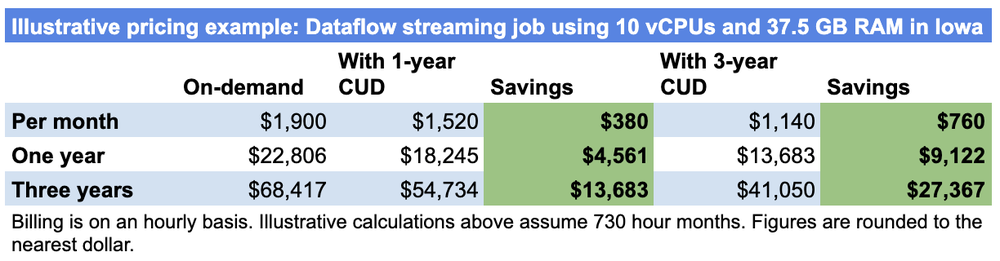
To illustrate how Dataflow streaming CUDs can help you save money, let’s look at an example. Let’s assume a Dataflow streaming job is running in us-central1 (Iowa). The streaming job in our example is using the following resources:
10 nodes of instance type n1-standard-1 (vCPUs: 1, RAM: 3.75 GB)
20 streaming engine compute units per hour
From the Dataflow pricing page, you can calculate the approximate hourly cost of your job to be $2.6034:
10 nodes * 1 streaming vCPU per node * $0.069 per streaming vCPU per hour = $0.69 per hour
10 nodes * 3.75GB per node * $0.003557 per GB per hour = $0.1334 per hour
20 streaming engine compute units * $0.089 per compute unit per hour = $1.78 per hour
(Please note that the above prices are examples. For current prices, see Dataflow pricing.)
If you purchase a one-year CUD for the same job, you will get a 20% discount. This means that the cost of the job will be reduced from $2.6034 to $2.0827 per hour. Over the course of a year, Dataflow streaming CUDs will help you save $4,561.33.
If you purchase a three-year CUD for the job, you will get a 40% discount. This means that the cost of the job will be reduced from $2.6034 to $1.562 per hour. Dataflow streaming CUDs will help you save $9122.31 annually, or $27,366.99 over the course of three years
When to use Dataflow streaming CUDs
Dataflow streaming CUDs are ideal for workloads with predictable resource needs like personalized product recommendations, predictive maintenance, and smart supply chains. As streaming jobs are expected to be used quite consistently, you can purchase Dataflow streaming CUDs to better manage the cost of your streaming jobs.
Dataflow streaming CUDs are also a good choice for workloads that are growing steadily, since bringing more workloads to Dataflow streaming increases the value that existing workloads can get from Dataflow streaming CUDs. For example, if you expect your streaming usage to grow by 30% each year, you can purchase a three-year Dataflow streaming CUD at your current usage levels to lock in a 40% discount. As your workload grows, you can purchase additional Dataflow streaming CUDs to maintain or grow your CUD utilization rate, and cover even more of your Dataflow streaming spend with attractive discounts.
How to purchase Dataflow streaming CUDs
To purchase a Dataflow streaming CUD, go to the committed use discounts page in the Cloud console. You can make your commitment based on the current usage patterns and projected growth of the streaming jobs that you would like to cover with your commitment. Once you choose your commitment period, you will see the cost of your commitment after the discounts and how much you’re saving. It’s that easy!
Take the next step
Dataflow provides a versatile, scalable and cost-effective platform to run your streaming workloads. With Dataflow streaming CUDs, you can save even more on your Dataflow costs! Check out our documentation and pricing page for more details on Dataflow streaming CUDs.
Data is a competitive advantage and customers in all industries are looking for complete, simplified business intelligence (BI) solutions to meet their specific needs. Every company, team, and individual wants to work with data to solve problems in their own way, with intuitive tools designed for today’s AI-driven landscape.
Our vision is to make Looker the most innovative and flexible AI-driven BI platform, with an integrated, simple and beautiful experience, enabling self-service analytics, governed reporting and embedded BI with a leading semantic model, across databases and clouds.
With Cloud Next 2024 rapidly approaching this April, we are set to provide even more updates on this journey. One of the most significant ways we will make progress on our goals in 2024 is by bringing Looker Studio together with Looker in a single unified product.
This new converged experience will enable all Looker customers to gain the benefits of Looker Studio’s visualization and analytical capabilities on top of their trusted data, and make available new self-service options. This combined offering, bringing self-service BI and governed modeled BI together, enables every stakeholder in an organization to leverage data in their own way, in a single, powerful managed platform.
A BI platform built for AI and more
For years, organizations of all types have chosen Looker as a way to surface trusted data at scale, to design data-driven applications and bring insights to all parts of the company. We’re extending this mission as gen AI is combined with BI and will continue to invest here to enable data-driven businesses to do more.
Looker’s API-first platform has set the stage for any workflow or application to connect to your data, from practically any source, with our semantic layer defining terms and ensuring the output is trusted. In 2024, we are extending Looker with deeper connections to Google Cloud and Workspace, including integration with Vertex AI, providing essential tools for users to build custom data applications. You can learn more about this plan, as well as our many recent feature releases, from our Looker Vision, Strategy, and Roadmap for 2024 webinar, where we outlined how we are helping customers accelerate time to insights with a modern, cloud-native platform.
As we showed in our product roadmap webcast, we continue to evolve Looker with a focus on simplicity and unification, while also gaining the benefits of gen AI, powered by large language models. We will have data systems speak the language of humans, and enable business users and data analysts to chat and interact with their business data, where they work.
What’s next? Find out at Next.
If you were unable to attend our roadmap presentation live, be sure you watch it on demand and hear directly from the product leadership team on our plans. We will be sharing the latest product news from Looker and gen AI, as well as showcasing customer innovations, at Google Cloud Next this April 9-11 in Las Vegas, Nevada. You won’t want to miss it.
Register today to see what’s Next and experience the new way to cloud.