Get to know BigQuery data canvas: an AI-centric experience to reimagine data analytics
Navigating the complexities of the data-to-insights journey can be frustrating. Data professionals spend valuable time sifting through data sources, reinventing the wheel with each new question that comes their way. They juggle multiple tools, hop between coding languages, and collaborate with a wide array of teams across their organizations. This fragmented approach is riddled with bottlenecks, preventing analysts from generating insights and doing high-impact work as quickly as they should.
Yesterday at Google Cloud Next ‘24, we introduced BigQuery data canvas, which reimagines how data professionals work with data. This novel user experience helps customers create graphical data workflows that map to their mental model while AI innovations accelerate finding, preparing, analyzing, visualizing and sharing data and insights.
Watch this video for a quick overview of BigQuery data canvas.
BigQuery data canvas: a NL-driven analytics experience
BigQuery data canvas makes data analytics faster and easier with a unified, natural language-driven experience that centralizes data discovery, preparation, querying, and visualization. Rather than toggling between multiple tools, you can now use data canvas to focus on the insights that matter most to your business. Data canvas addresses the challenges of traditional data analysis workflow in two areas:
Natural language-centric experience: Instead of writing code, you can now speak directly to your data. Ask questions, direct tasks, and let the AI guide you through various analytics tasks.
Reimagined user experience: Data canvas rethinks the notebook concept. Its expansive canvas workspace fosters iteration and easy collaboration, allowing you to refine your work, chain results, and share workspaces with colleagues.
For example, to analyze a recent marketing campaign with BigQuery data canvas, you could use natural language prompts to discover campaign data sources, integrate them with existing customer data, derive insights, collaborate with teammates and share visual reports with executives — all within a single canvas experience.
Natural language-based visual workflow with BigQuery data canvas
Do more with BigQuery data canvas
BigQuery provides a variety of features that can help analysts accelerate their analytics tasks:
Search and discover: Easily find the specific data asset visualization table or view that you need to work with. Or search for the most relevant data assets. Data canvas works with all data that can be managed with BigQuery, including BigQuery managed storage, BigLake, Google Cloud Storage objects, and BigQuery Omni tables. For example, you could use either of the follow inputs to pull data with data canvas:
Specific table: project_name.dataset_name.table_name
Search: “customer transaction data” or “projectid:my-project-name winter jacket sales Atlanta”
Explore data assets: Review the table schema, review their details or preview data and compare it side by side.
Generate SQL queries: Iterate with NL inputs to generate the exact SQL query you need to accomplish the analytics task at hand. You can also edit the SQL before executing it.
Combine results: Define joins with plain language instructions and refine the generated SQL as needed. Use query results as a starting point for further analysis with prompts like “Join this data with our customer demographics on order id.”
Visualize: Use natural language prompts to easily create and customize charts and graphs to visualize your data, e.g., “create a bar chart with gradient” Then, seamlessly share your findings by exporting your results to Looker Studio or Google Sheets.
Automated insights: Data canvas can interpret query results and chart data and generate automated insights from them. For example, it can look at the query results of sales deal sizes and automatically provide the insight “the median deal size is $73,500.”
Share to collaborate: Data analytics projects are often a team effort. You can simply save your canvas and share it with others using a link.
Popular use cases
While BigQuery data canvas can accelerate many analytics tasks, it’s particularly helpful for:
Ad hoc analysis: When working on a tight deadline, data canvas makes it easy to pull data from various sources.
Exploratory data analysis (EDA): This critical early step in the data analysis process focuses on summarizing the main characteristics of a dataset, often visually. Data canvas helps find data sources and then presents the results visually.
Collaboration: Data canvas makes it easy to share an analytics project with multiple people.
What our customers are saying
Companies large and small have been experimenting with BigQuery data canvas for their day-to-day analytics tasks and their feedback has been very positive.
Wunderkind, a performance marketing channel that powers one-to-one customer interactions, has been using BigQuery data canvas across their analytics team for several weeks and is experiencing significant time savings.
“For any sort of investigation or exploratory exercise resulting in multiple queries there really is no replacement [for data canvas]. [It] Saves us so much time and mental capacity!” – Scott Schaen, VP of Data & Analytics, Wunderkind
Veo, a micro mobility company that operates in 50+ locations across the USA, is seeing immediate benefits from the AI capabilities in data canvas.
“I think it’s been great in terms of being able to turn ideas in the form of NL to SQL to derive insights. And the best part is that I can review and edit the query before running it – that’s a very smart and responsible design. It gives me the space to confirm it and ensure accuracy as well as reliability!” – Tim Velasquez, Head of Analytics, Veo
Give BigQuery data canvas a try
To learn more, watch this video and check out the documentation. BigQuery data canvas is launching in preview and will be rolled out to all users starting on April 15th. Submit this form to get early access.
For any bugs and feedback, please reach out to the product and engineering team at datacanvas-feedback@google.com. We’re looking forward to hearing how you use the new data canvas!
Source : Data Analytics Read More