Connecting one messaging system to another messaging system can be difficult. While many options exist, such as managed connectors, DIY connectors, and Dataflow jobs, we’re always exploring ways to make moving data even simpler.
Today, the Pub/Sub Lite team is excited to introduce export subscriptions that can write messages from a Lite topic directly to a destination Pub/Sub topic. Export subscriptions can be used for migration from Pub/Sub Lite to Pub/Sub, increasing interoperability between teams with different messaging system needs, and consolidating or connecting data pipelines.
Export subscriptions are a subtype of Lite subscriptions; there are standard subscriptions and export subscriptions. Export subscriptions require a destination. When you set an export subscription’s destination to Pub/Sub, a Lite topic can connect directly to a Pub/Sub topic.
An export subscription can only write to one Pub/Sub topic, but different messaging patterns are supported. For fan-in, you can create multiple export subscriptions that all write to the same destination Pub/Sub topic. For fan-out, you can create multiple export subscriptions that all originate from the same Lite topic but each write to a different destination Pub/Sub topic. Other notable features of export subscriptions to destination Pub/Sub include the ability to change the destination Pub/Sub topic on an existing export subscription, optionally configuring a dead letter Lite topic to retain incompatible or oversized messages, and cross-project exporting.
An export subscription not only acts like a regular Pub/Sub Lite subscriber but also acts as a Pub/Sub publisher. Just like standard Lite subscriptions, export subscriptions consume Lite subscription throughput capacity. Export subscriptions also incur Pub/Sub publish throughput usage. In other words, existing Pub/Sub Lite and Pub/Sub charges continue to apply, but the export is provided by the service at no additional cost. See Pub/Sub pricing page for details.
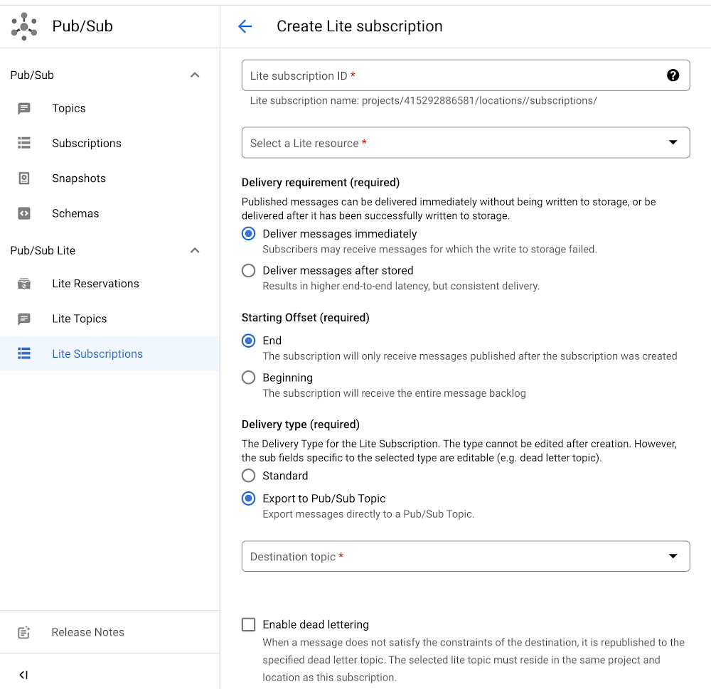
Export subscriptions help create a seamless Pub/Sub ecosystem and increase compatibility between GCP products. You can create an export subscription to a destination Pub/Sub topic via gCloud (CLI), Cloud Console (UI), and API. Get started today by going to ‘Pub/Sub’ in the Cloud Console, selecting ‘Lite Subscriptions’ on the left hand navigation, clicking ‘Create Lite Subscription’ on the top navigation bar, and then setting ‘Delivery Type’ to ‘Export to Pub/Sub topic.’
Transactions are mission critical for modern enterprises supporting payments, logistics, and a multitude of business operations. And in today’s modern analytics-first and data-driven era, the need for the reliable processing of complex transactions extends beyond just the traditional OLTP database; today businesses also have to trust that their analytics environments are processing transactional data in an atomic, consistent, isolated, and durable (ACID) manner. So BigQuery set out to support DML statements spanning large numbers of tables in a single transaction and commit the associated changes atomically (all at once) if successful or rollback atomically upon failure. And today, we’d like to highlight the recent general availability launch of multi-statement transactions within BigQuery and the new business capabilities it unlocks.
While in preview, BigQuery multi-statement transactions were tremendously effective for customer use cases, such as keeping BigQuery synchronized with data stored in OLTP environments, the complex post processing of events pre-ingested into BigQuery, complying with GDPR’s right to be forgotten, etc. One of our customers, PLAID, leverages these multi-statement transactions within their customer experience platform KARTE to analyze the behavior and emotions of website visitors and application users, enabling businesses to deliver relevant communications in real time and further PLAID’s mission to Maximize the Value of People with the Power of Data.
“We see multi-statement transactions as a valuable feature for achieving expressive and fast analytics capabilities. For developers, it keeps queries simple and less hassle in error handling, and for users, it always gives reliable results.”—Takuya Ogawa, Lead Product Engineer
The general availability of multi-statement transactions not only provides customers with a production ready means of handling their business critical transactions in a comprehensive manner within a single transaction, but now also provides customers with far greater scalability compared to what was offered during the preview. At GA, multi-statement transactions increase support for mutating up to 100,000 table partitions and modifying up to 100 tables per transaction. This 10x scale in the number of table partitions and 2x scale in the number of tables was made possible by a careful re-design of our transaction commit protocol which optimizes the size of the transactionally committed metadata.
The GA of multi-statement transactions also introduces full compatibility with BigQuery sessions and procedural language scripting. Sessions are useful because they store state and enable the use of temporary tables and variables, which then can be run across multiple queries when combined with multi-statement transactions. Procedural language scripting provides users the ability to run multiple statements in a sequence with shared state and with complex logic using programming constructs such as IF … THEN and WHILE loops.
For instance, let’s say we wanted to enhance the current multi-statement transaction example, which uses transactions to atomically manage the existing inventory and supply of new arrivals of a retail company. Since we’re a retailer monitoring our current inventory on hand, we would now also like to add functionality to automatically suggest to our Sales team which items we should promote with sales offers when our inventory becomes too large. To do this, it would be useful to include a simple procedural IF statement, which monitors the current inventory and supply of new arrivals and modifies a new PromotionalSales table based on total inventory levels. And let’s validate the results ourselves before committing them as one single transaction to our sales team by using sessions. Let’s see how we’d do this via SQL.
First, we’ll create our tables using DDL statements:
code_block[StructValue([(u’code’, u’CREATE OR REPLACE TABLE my_dataset.Inventoryrn(product string,rnquantity int64,rnsupply_constrained bool);rn rnCREATE OR REPLACE TABLE my_dataset.NewArrivalsrn(product string,rnquantity int64,rnwarehouse string);rn rnCREATE OR REPLACE TABLE my_dataset.PromotionalSalesrn(product string,rninventory_on_hand int64,rnexcess_inventory int64);’), (u’language’, u”), (u’caption’, <wagtail.wagtailcore.rich_text.RichText object at 0x3ed8efa027d0>)])]
Then, we’ll insert some values into our Inventory and NewArrivals tables:
Now, we’ll use a multi-statement transaction and procedural language scripting to atomically merge our NewArrivals table with the Inventory table while taking excess inventory into account to build out our PromotionalSales table. We’ll also create this within a session, which will allow us to validate the tables ourselves before committing the statement to everyone else.
code_block[StructValue([(u’code’, u”DECLARE average_product_quantity FLOAT64;rn rnBEGIN TRANSACTION;rn rnCREATE TEMP TABLE tmp AS SELECT * FROM my_dataset.NewArrivals WHERE warehouse = ‘warehouse #1’;rnDELETE my_dataset.NewArrivals WHERE warehouse = ‘warehouse #1′;rn rn#Calculates the average of all product inventories.rnset average_product_quantity = (SELECT AVG(quantity) FROM my_dataset.Inventory);rn rnMERGE my_dataset.Inventory IrnUSING tmp TrnON I.product = T.productrnWHEN NOT MATCHED THENrnINSERT(product, quantity, supply_constrained)rnVALUES(product, quantity, false)rnWHEN MATCHED THENrnUPDATE SET quantity = I.quantity + T.quantity;rn rn#The below procedural script uses a very simple approach to determine excess_inventory based on current inventory being 120% of the average inventory across all products.rnIF EXISTS(SELECT * FROM my_dataset.Inventoryrn WHERE quantity > (1.2 * average_product_quantity)) THENrn INSERT my_dataset.PromotionalSales (product, inventory_on_hand, excess_inventory)rn SELECTrn product,rn quantity as inventory_on_hand,rn quantity – CAST(ROUND((1.2 * average_product_quantity),0) AS INT64) as excess_inventoryrn FROM my_dataset.Inventoryrn WHERE quantity > (1.2 * average_product_quantity);rnEND IF;rn rnSELECT * FROM my_dataset.NewArrivals;rnSELECT * FROM my_dataset.Inventory ORDER BY product;rnSELECT * FROM my_dataset.PromotionalSales ORDER BY excess_inventory DESC;rn#Note the multi-statement SQL temporarily stops here within the session. This runs successfully if you’ve set your SQL to run within a session.”), (u’language’, u”), (u’caption’, <wagtail.wagtailcore.rich_text.RichText object at 0x3ed900d72b50>)])]
From the results of the SELECT statements, we can see the warehouse #1 arrivals were successfully added to our inventory and the PromotionalSales table correctly reflects what excess inventory we have. Looks like these transactions are ready to be committed.
However, just in case there were some issues with our expected results, if others were to query the tables outside the session we created, the changes wouldn’t have taken effect. Thus, we have the ability to validate our results and could roll them back if needed without impacting others.
code_block[StructValue([(u’code’, u’#Run in a different tab outside the current session. Results displayed will be consistent with the tables before running the multi-statement transaction.rnSELECT * FROM my_dataset.NewArrivals;rnSELECT * FROM my_dataset.Inventory ORDER BY product;rnSELECT * FROM my_dataset.PromotionalSales ORDER BY excess_inventory DESC;’), (u’language’, u”), (u’caption’, <wagtail.wagtailcore.rich_text.RichText object at 0x3ed901a59050>)])]
Going back to our configured session, since we’ve validated our Inventory, NewArrivals, and PromotionalSales tables are correct, we can go ahead and commit the multi-statement transaction within the session, which will propagate the changes outside the session too.
code_block[StructValue([(u’code’, u’#Now commit the transaction within the same session configured earlier. Be sure to delete or comment out the rest of the SQL text run earlier.rnCOMMIT TRANSACTION;’), (u’language’, u”), (u’caption’, <wagtail.wagtailcore.rich_text.RichText object at 0x3ed901c9ff90>)])]
And now that the PromotionalSales table has been updated for all users, our sales team has some ideas of what products they should promote due to our excess inventory.
code_block[StructValue([(u’code’, u’#Results now propagated for all users.rnSELECT * FROM my_dataset.PromotionalSales ORDER BY excess_inventory DESC;’), (u’language’, u”), (u’caption’, <wagtail.wagtailcore.rich_text.RichText object at 0x3ed8ef2034d0>)])]
As you can tell, using multi-statement transactions is simple, scalable, and quite powerful, especially combined with other BigQuery Features. Give them a try yourself and see what’s possible.
Powered by Vertex AI (Google Cloud’s platform for accelerating development and deployment of machine learning models into production), SAVI (Semi Automated Vision Inspection)1 is transforming surgical instrument identification and cataloging, leading to fewer canceled surgeries and easing pressure on surgery waitlists.
Max Kelsen, an analytics and software agency that specializes in machine learning, has worked closely with Google Cloud and Johnson & Johnson MedTech to create a system that can manage tens of thousands of individual devices, their characteristics, and how they apply to each set or tray used by a surgeon. SAVI does this while delivering a one in 10,000 real-world error rate, much faster and more accurately than manual processes currently in use across the industry. Implementing SAVI can also unlock end-to-end visibility and traceability across the surgical set supply chain and provide advanced analytics and insights.
Eliminating time-consuming manual processes
Surgeons need a large number of specialist instruments and devices to complete complex, delicate procedures. Because each tray of these instruments can typically cost more than $350,000, and having every type of set on shelf at every surgical facility is not feasible, manufacturers generally loan them to hospitals for procedures, such as inserting one of the manufacturers’ implants into a patient’s knee. Once a procedure is complete, the hospital returns the instrument tray to the manufacturer for storage and re-distribution to other hospitals as needed.
Each time a hospital returns a tray, the manufacturer needs to check that each instrument is there, correctly placed, cleaned, and fit for the purpose of the next procedure. As each set may hold more than 400 instruments, completing this process manually is complex and time-consuming. While each tray is checked before and after surgery at the hospital, and again when it arrives and leaves the manufacturer’s facility, Max Kelsen finds that 5% of surgeries can still be affected by missing, broken or bent instruments. This has a severe downstream impact on private hospitals in particular, directly affecting patient safety and outcomes; in Australia, for example, around 60% of surgeries are performed in private hospitals.
Johnson & Johnson MedTech has 60,000 surgical trays across the Asia-Pacific, and loans these trays out about 100,000 times per month. The manufacturer approached Max Kelsen to help design and develop a solution to make the supply chain more efficient, and to give more visibility into asset movement. As a Google Cloud Partner specializing in applying machine learning at scale in healthcare contexts, Max Kelsen had the expertise and track record to meet Johnson & Johnson MedTech’s need for a globally scalable solution that was engineered for quality and performance.
The first step was to establish a baseline for the project by determining how long the manufacturer’s team took to process each tray, and to set an efficiency number. We then spent six months determining and evaluating how to deliver a robust, accurate solution that outperformed current manual and labor-intensive methods in processing instruments and trays, globally. Our work included extensive technical feasibility research involving a representative sample for the variety and complexity of sets, trays, and devices needed for different types of surgery, including orthopedics, spinal trauma, and maxillofacial groups.
Working with Google Cloud to accelerate and de-risk the project
This is a familiar problem that is industry-wide. The issue has been widely explored and tried with a number of technologies over several years without producing the scalability and performance results required to make this an appropriate and feasible solution. Google Cloud partnered with Max Kelsen to accelerate and de-risk this large and strategic project for a mutual customer.
Technical feasibility took four months, prior to a year-long production pilot of SAVl in a distribution center in Queensland that services over 100 hospitals. After obtaining enough real-world data and experience to validate that the solution was as scalable and as accurate as needed, an Asia-Pacific rollout of the system commenced. SAVI is now live across Johnson & Johnson MedTech’s operations in Australia, New Zealand, and Japan, garnering recognition with a JAISA excellence award.
Google Cloud machine learning is integral to SAVI. Google Cloud’s technologies were a big differentiator for Max Kelsen’s engineering team in delivering the breakthroughs needed at scale, and in production, to meet Johnson & Johnson MedTech’s needs.
Reducing checking and documentation time
Running SAVI in Google Cloud has reduced the time Johnson & Johnson MedTech needs to check and document inspections of these surgical instrument sets by over 40%. The application also delivers consistent measurable quality that is often hard to measure at scale when using manual processes. During the pandemic, the application enabled Johnson & Johnson MedTech to operate with a lower headcount for the same volume output, enabling the organization to quickly service a backlog of waiting list surgeries.
In addition, the automation delivered with SAVI has reduced the time required to bring technicians up to speed on quality control processes, from eight to 12 months down to just three months, enhancing productivity and performance while delivering a more robust workforce.
So how does SAVI work in a real-world context? SAVI is deployed via a tablet and a web-based application incorporates an API to photograph the medical device trays, as shown below. Max Kelsen captures the photograph and sends it to a range of different services, via an API endpoint hosted on Google Cloud:
Once this tray and device onboarding stage is completed, the next step is to perform inferences from the images and data. By hosting online models with Kubeflow model serving on GKE, we enable a model to identify all the instruments in a tray at low latency.
Vertex AI Workbench notebooks are used for data exploration and modeling. Kubeflow training pipelines hosted on GKE are executed to produce machine learning models for specific surgical instrument sets. Several hundred machine learning models are then hosted with Kubeflow model serving on GKE, with state and analytics managed using Firebase. Using machine learning to infer from images whether any devices are incorrectly placed, dirty, or otherwise not fit for purpose, the data is then returned to the tablet for the user to respond accordingly.
Based on our success to date with SAVI, it is now available on Google Cloud Marketplace to help healthcare organizations achieve machine learning-powered efficiencies across a range of use cases, and ultimately improve patient safety and outcomes.
1. Not to be confused with the usage of Visual Inspection Model (Assembly) available in Vertex AI Vision
To produce any sufficiently accurate machine learning model, the process requires tuning parameters and hyperparameters. Your model’s parameters are variables that your chosen machine learning technique uses to adjust to your data, like weights in neural networks to minimize loss. Hyperparameters are variables that control the training process itself. For example, in a multilayer perceptron, altering the number and size of hidden layers can have a profound effect on your model’s performance, as does the maximum depth or minimum observations per node in a decision tree.
Hyperparameter tuning can be a costly endeavor, especially when done manually or when using exhaustive grid search to search over a larger hyperparameter space.
In 2017, Google introduced Vizier, a technique used internally at Google for performing black-box optimization. Vizier is used to optimize many of our own machine learning models, and is also available in Vertex AI, Google Cloud’s machine learning platform. Vertex AI Hyperparameter tuning for custom training is a built-in feature using Vertex AI Vizier for training jobs. It helps determine the best hyperparameter settings for an ML model.
Overview
In this blog post, you will learn how to perform hyperparameter tuning of your custom R models through Vertex AI.
Since many R users prefer to use Vertex AI from RStudio programmatically, you will interact with Vertex AI through the Vertex AI SDK via the reticulate package.
The process of tuning your custom R models on Vertex AI comprises the following steps:
Enable Google Cloud Platform (GCP) APIs and set up the local environment
Create custom R script for training a model using specific set of hyperparameters
Create a Docker container that supports training R models with Cloud Build and Container Registry
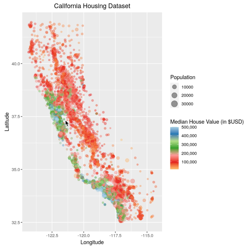
To showcase this process, you train a simple boosted tree model to predict housing prices on the California housing data set. The data contains information from the 1990 California census. The data set is publicly available from Google Cloud Storage at gs://cloud-samples-data/ai-platform-unified/datasets/tabular/california-housing-tabular-regression.csv
The tree model model will predict a median housing price, given a longitude and latitude along with data from the corresponding census block group. A block group is the smallest geographical unit for which the U.S. Census Bureau publishes sample data (a block group typically has a population of 600 to 3,000 people).
Environment setup
This blog post assumes that you are either using Vertex AI Workbench with an R kernel or RStudio. Your environment should include the following requirements:
The Google Cloud SDK
Git
R
Python 3
Virtualenv
To execute shell commands, define a helper function:
Next, you define variables to support the training and deployment process, namely:
PROJECT_ID: Your Google Cloud Platform Project ID
REGION: Currently, the regions us-central1, europe-west4, and asia-east1 are supported for Vertex AI; it is recommended that you choose the region closest to you
BUCKET_URI: The staging bucket where all the data associated with your dataset and model resources are stored
DOCKER_REPO: The Docker repository name to store container artifacts
IMAGE_NAME: The name of the container image
IMAGE_TAG: The image tag that Vertex AI will use
IMAGE_URI: The complete URI of the container image
When you initialize the Vertex AI SDK for Python, you specify a Cloud Storage staging bucket. The staging bucket is where all the data associated with your dataset and model resources are retained across sessions.
Create container images for training and tuning models
The Dockerfile for your custom container is built on top of the Deep Learning container — the same container that is also used for Vertex AI Workbench. You just add an R script for model training and tuning.
Before creating such a container, you enable Artifact Registry and configure Docker to authenticate requests to it in your region.
code_block[StructValue([(u’code’, u’# filename: Dockerfile – container specifications for using R in Vertex AIrnFROM gcr.io/deeplearning-platform-release/r-cpu.4-1:latestrnrnWORKDIR /rootrnrnCOPY train.R /root/train.Rrnrn# Install FortranrnRUN apt-get updaternRUN apt-get install gfortran -yyrnrn# Install R packagesrnRUN Rscript -e \”install.packages(‘plumber’)\”rnRUN Rscript -e \”install.packages(‘argparser’)\”rnRUN Rscript -e \”install.packages(‘gbm’)\”rnRUN Rscript -e \”install.packages(‘caret’)\”rnRUN Rscript -e \”install.packages(‘reticulate’)\”rnrnRUN pip install cloudml-hypertune’), (u’language’, u”), (u’caption’, <wagtail.wagtailcore.rich_text.RichText object at 0x3ef172d55950>)])]
Next, create the file train.R, which is used to train your R model. The script trains a gbm model (generalized boosted regression model) on the California Housing dataset. Vertex AI sets environment variables that you can utilize, and the hyperparameters for each trial are passed as command line arguments. The trained model artifacts are then stored in your Cloud Storage bucket. The results of your training script are communicated back to Vertex AI using the hypertune package, which stores a JSON file to /tmp/hypertune/output.metrics. Vertex AI uses this information to come up with a hyperparameter configuration for the next trial, and to assess which trial was responsible for the best overall result.
code_block[StructValue([(u’code’, u’#!/usr/bin/env Rscriptrn# filename: train.R – perform hyperparameter tuning on a boosted tree model using Vertex AIrnrnlibrary(tidyverse)rnlibrary(data.table)rnlibrary(argparser)rnlibrary(jsonlite)rnlibrary(reticulate)rnlibrary(caret)rnrn# The GCP Project IDrnproject_id <- Sys.getenv(“CLOUD_ML_PROJECT_ID”)rnrn# The GCP Regionrnlocation <- Sys.getenv(“CLOUD_ML_REGION”)rnrn# The Cloud Storage URI to upload the trained model artifact tornmodel_dir <- Sys.getenv(“AIP_MODEL_DIR”)rnrn# The trial IDrntrial_id <- Sys.getenv(“CLOUD_ML_TRIAL_ID”, 0)rnrn# The JSON file to save metric results tornmetric_file <- “/var/hypertune/output.metrics”rnrn# Read hyperparameters for this trialrnp <- arg_parser(“California Housing Model”) %>%rn add_argument(“–n.trees”, default = “100”, help = “number of trees to fit”, type = “integer”) %>%rn add_argument(“–interaction.depth”, default = 3, help = “maximum depth of each tree”) %>%rn add_argument(“–n.minobsinnode”, default = 10, help = “minimun number of observations in terminal node”) %>%rn add_argument(“–shrinkage”, default = 0.1, help = “learning rate”) %>%rn add_argument(“–data”, help = “path to the training data in GCS”)rnrndir.create(“/tmp/hypertune”)rnargv <- parse_args(p, unlist(strsplit(commandArgs(trailingOnly = TRUE), “=”)))rnrnrn# Read housing datasetrnsystem2(“gsutil”, c(“cp”, argv$data, “./data.csv”))rndata <- fread(“data.csv”)rnprint(data)rnrnrn# Start model training with the hyperparameter for the trialrnprint(“Starting Model Training”)rntuneGrid <- expand.grid(rn interaction.depth = as.integer(argv$interaction.depth),rn n.trees = as.integer(argv$n.trees),rn n.minobsinnode = as.integer(argv$n.minobsinnode),rn shrinkage = as.numeric(0.1)rn)rnprint(tuneGrid)rnfitControl <- trainControl(method = “cv”, number = 3)rnset.seed(42)rnfit <- train(median_house_value ~ .,rn method = “gbm”,rn trControl = fitControl,rn tuneGrid = tuneGrid,rn metric = “MAE”,rn data = datarn)rnrnmean_absolute_error <- mean(fit$resample$MAE)rncat(paste(“mean absolute error:”, mean_absolute_error, “\\n”))rnrnrn# Report hyperparameter tuning metric to Vertex AI for pickingrn# hyperparameter configuration for the next trialrnhypertune <- import(“hypertune”)rnhpt <- hypertune$HyperTune()rnhpt$report_hyperparameter_tuning_metric(rn hyperparameter_metric_tag = “mean_absolute_error”,rn metric_value = as.numeric(mean_absolute_error),rn global_step = 1000)rnrnrn# Save model to Cloud Storage bucketrnsaveRDS(fit$finalModel, “gbm.rds”)rnsystem2(“gsutil”, c(“cp”, “gbm.rds”, model_dir))’), (u’language’, u”), (u’caption’, <wagtail.wagtailcore.rich_text.RichText object at 0x3ef17393a590>)])]
Finally, you build the Docker container image on Cloud Build – the serverless CI/CD platform. Building the Docker container image may take 10 to 15 minutes.
Once your training application is containerized, you define the machine specifications for the tuning job. In this example, you use n1-standard-4 instances.
Hyperparameter tuning jobs search for the best combination of hyperparameters to optimize your metrics. Hyperparameter tuning jobs do this by running multiple trials of your training application with different sets of hyperparameters.
You can control the job in the following ways:
max_trial_count: Decide how many trials you want to allow the service to run. Increasing the number of trials generally yields better results, but it is not always so. Usually, there is a point of diminishing returns after which additional trials have little or no effect on the accuracy. Before starting a job with a large number of trials, you may want to start with a small number of trials to gauge the effect your chosen hyperparameters have on your model’s accuracy. To get the most out of hyperparameter tuning, you shouldn’t set your maximum value lower than ten times the number of hyperparameters you use.
parallel_trial_count: You can specify how many trials can run in parallel. Running parallel trials has the benefit of reducing the time the training job takes (real time — the total processing time required is not typically changed). However, running in parallel can reduce the effectiveness of the tuning job overall. That is because hyperparameter tuning uses the results of previous trials to inform the values to assign to the hyperparameters of subsequent trials. When running in parallel, some trials start without having the benefit of the results of any trials still running.
In addition, you also need to specify which hyperparameters to tune. There is little universal advice to give about how to choose which hyperparameters you should tune. If you have experience with the machine learning technique that you’re using, you may have insight into how its hyperparameters behave. You may also be able to find advice from machine learning communities.
However you choose them, it’s important to understand the implications. Every hyperparameter that you choose to tune has the potential to increase the number of trials required for a successful tuning job. When you run a hyperparameter tuning job on Vertex AI, the amount you are charged is based on the duration of the trials initiated by your hyperparameter tuning job. A careful choice of hyperparameters to tune can reduce the time and cost of your hyperparameter tuning job.
The results of this tuning job can also be inspected from the Vertex AI Console.
Summary
In this blog post, you have gone through tuning a custom R model using Vertex AI. For easier reproducibility, you can refer to this notebook on GitHub. You can deploy the resultant model from the best trial on Vertex AI Prediction following the article here.
We’re excited to share that Gartner has recognized Google as a Leader in the 2022 Gartner® Magic Quadrant™ for Cloud Database Management Systems, for the third year in a row. We believe this recognition is a testimony to Google Cloud’s vision and strong track record of delivering continuous product innovation, especially in areas like open data ecosystems and unified data cloud offerings.
Download the complimentary 2022 Gartner Magic Quadrant for Cloud Database Management Systems report.
Modern applications need to support a large number of globally distributed users, with no downtime and fast performance. And, with the exponential growth in the amount and types of data, workloads, and users, it’s becoming incredibly complex to harness data’s full potential.
This results in a growing data-to-value gap.
Google’s data cloud is well positioned to address the modern data needs of organizations with intelligent data and analytics services, advanced security, and a strong partner ecosystem, all integrated within a unified platform. We continue to rapidly innovate across these areas of the data space, especially with the new capabilities we announced at Google Cloud Next ’22 from our databases and data analytics portfolios.
Organizations such as Walmart, PayPal, and Carrefour, as well as tens of thousands of other customers around the world, have partnered with Google Cloud to drive innovation with a unified, open, and intelligent data ecosystem.
Unified data management
Google’s data cloud provides an open and unified data platform that allows organizations to manage every stage of the data lifecycle — from running operational databases for applications to managing analytical workloads across data warehouses and data lakes, to data-driven decision making, to AI and Machine Learning. The way we’ve architected our platform is truly unique and enables customers to bring together their data, their people and their workloads.
Our databases are built on a highly scalable distributed storage with fully disaggregated resources and high-performance Google-owned global networking. This combination allows us to provide tightly integrated data cloud services across our data cloud products such as Cloud Spanner, Cloud Bigtable, AlloyDB for PostgreSQL, BigQuery, Dataproc and Dataflow.
We recently launched several capabilities that further strengthen these integrations, making it even more seamless and easy for customers to accelerate innovation:
The unification of transactional and analytical systems. With change streams, customers can track writes, updates, and deletes to Spanner and Bigtable databases and replicate them to downstream systems such as BigQuery, Pub/Sub, and Cloud Storage. Datastream for BigQuery provides easy replication from operational database sources such as AlloyDB, PostgreSQL, MySQL, and Oracle, directly into BigQuery. This allows you to easily set up an ELT (Extract, Load, Transform) pipeline for low-latency data replication enabling real-time insights.
The unification of data of all types. BigLake enables customers to work with data of any type, in any location. Customers no longer have to worry about underlying storage formats and can reduce cost and inefficiencies because BigLake extends up from BigQuery. This level of integration allowed us to rapidly ship object tables, a new table type that provides a structured interface for unstructured data. Powered by BigLake, object tables let customers run analytics and ML on images, audio, documents natively, changing the game for data teams worldwide, who can now innovate without limits with all their data, in one unified environment.
The unification of workloads. We’ve introduced new developer extensions for workloads that require programming beyond SQL. With BigQuery stored procedures for Apache Spark, customers can run Spark programs directly from within BigQuery, unifying transformation and ingestion and enabling Spark procedures to run as a step in a set of SQL statements. This unification not only increases productivity but it also brings costs and billing benefits as customers only pay for the Spark job duration and resources consumed. And the costs are converted to either BigQuery bytes processed or BigQuery slots, giving customers a single billing unit for both data lake and data warehouse jobs.
Open data ecosystem
Google Cloud provides industry leading integration with open source and open APIs, which ensures portability, flexibility, and reduces the risk of vendor lock-in. We see customers like PayPal, HSBC, Vodafone, Major League Baseball and hundreds of others increasingly leverage our suite of migration services to power their data cloud transformation journey. This includes BigQuery Migration Service to accelerate migration from traditional data warehouses and the comprehensive Database Migration Program to accelerate migrations to the cloud with the right expertise, assessments and financial support. Customers can also take advantage of our managed services that are fully compatible with the most popular open source engines such as PostgreSQL , MySQL, and Redis.
And we don’t stop there. We also offer BigQuery Omni which enables insights beyond Google Cloud to data in other cloud environments, while providing a single pane of glass for analysis, governance, and security.
We continue to focus on making Google Cloud the most open data cloud that can unlock the full potential of data and remove the barriers to digital transformation. Some recent launches in this area include:
Modernize your PostgreSQL environment. Database Migration Service now supports migrations of any PostgreSQL database to AlloyDB, in an easy-to-use, secure, and serverless manner, and with minimal downtime.
Build an open format data lake. To support data openness, we announced the general availability of BigLake, to help you break down data silos by unifying lakes and warehouses. BigLake innovations add support for Apache Iceberg, which is becoming the standard for open source table format for data lakes. And soon, we’ll add support for formats including Delta Lake and Hudi.
Bring analytics to your data. To help you analyze data irrespective of where it resides, we launched BigQuery Omni. Now we’re adding new capabilities such as cross-cloud transfer and cross-cloud larger query results that will make it easier to combine and analyze data across cloud environments.
We’ve significantly expanded our data cloud partner ecosystem, and are increasing our partner investments across many new areas. Today, more than 800 software partners are building their products using Google’s data cloud, and more than 40 data platform partners offer validated integrations through our Google Cloud Ready – BigQuery initiative. Earlier this year we launched the Data Cloud Alliance, now supported by 17 leaders in data working together to promote open standards and interoperability between popular data applications. We also announced a major expansion of the AlloyDB partner ecosystem, with more than 30 partner solutions to support business intelligence, analytics, data governance, observability, and system integration.
AI-powered innovation
At Google, AI is in our DNA. For two decades, we’ve leveraged the power of AI to organize the world’s information and make it useful to people and businesses everywhere. From enhancing the performance of our Search algorithm with ML, to sharpening content recommendations on YouTube with unsupervised learning, we have constantly leveraged AI to solve some of the toughest challenges in the market.
We continue to bring that same expertise in AI technology to make our data cloud services even more intelligent.
Database system optimizations. Capabilities such as Cloud SQL recommenders and AlloyDB autopilot make it easier for database administrators and DevOps teams to manage performance and cost for large fleets of databases.
Databases and AI integration. In addition to infusing AI and ML into our products, we have tightly integrated Spanner, AlloyDB and BigQuery with Vertex AI to simplify the ML experience. With these integrations, AlloyDB and Spanner users can now enable model inferencing directly within the database transaction using SQL.
Simplified ML Ops. Models created in BigQuery using BigQuery ML are now instantly visible in Vertex AI model registry. You can then directly deploy these models to Vertex AI endpoints for real-time serving, use Vertex AI pipelines to monitor and train models and view detailed explanations for your predictions through BigQuery ML and Vertex AI integration.
Google Cloud databases and analytics solutions are proven to operate at scale. For example, Spanner processes over 2 billion requests per second at peak, and BigQuery customers analyze over 110 terabytes of data per second.
We are honored to be a Leader in the 2022 Gartner Magic Quadrant for Cloud Database Management Systems, and look forward to continuing to innovate and partner with you on your digital transformation journey.
Download the complimentary 2022 Gartner Magic Quadrant for Cloud Database Management Systems report.
Gartner Magic Quadrant for Cloud Database Management Systems, Henry Cook, Merv Adrian, Rick Greenwald, Xingyu Gu, December 13, 2022 GARTNER is a registered trademark and service mark, and MAGIC QUADRANT is a registered trademark of Gartner, Inc. and/or its affiliates in the U.S. and internationally and are used herein with permission. All rights reserved. Gartner does not endorse any vendor, product or service depicted in its research publications, and does not advise technology users to select only those vendors with the highest ratings or other designation. Gartner research publications consist of the opinions of Gartner’s research organization and should not be construed as statements of fact. Gartner disclaims all warranties, expressed or implied, with respect to this research, including any warranties of merchantability or fitness for a particular purpose.
This graphic was published by Gartner, Inc. as part of a larger research document and should be evaluated in the context of the entire document. The Gartner document is available upon request from Google.
Unlocking the full potential of data requires breaking down the silo between open-source data formats and data warehouses. At the same time, it is critical to enable data governance team to apply policies regardless of where the data happens, whether – on file or columnar storage.
Today, data governance teams have to become subject matter experts on each storage system the corporate data happens to reside on. Since February 2022, Dataplex has offered a unified place to apply policies, which are propagated across both lake storage and data warehouses in GCP. Rather than specifying policies in multiple places, bearing the cognitive load of translating policies from “what you want the storage system to do” to “how your data should behave” Dataplex offers a single point for unambiguous policy management. Now, we are making it easier for you to use BigLake.
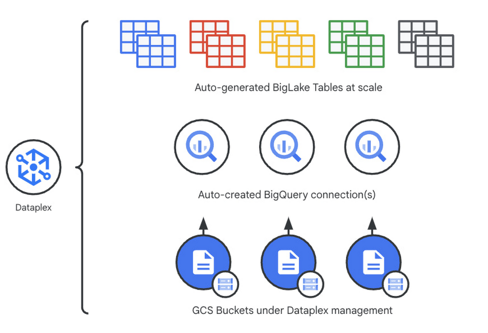
Earlier this year, we launched BigLake into general availability, BigLake unifies data fabric between Data Lakes and Data Warehouses by extending BigQuery storage to open file formats. Today, we announce BigLake Integration with Dataplex (available in preview). This integration eliminates the configuration steps for the admin taking advantage of BigLake and managing policies across GCS and BigQuery from a unified console.
Previously, you could point Dataplex at a Google Cloud Storage (GCS) bucket, and Dataplex will discover and extract all metadata from the data lake and register this metadata in BigQuery (and Dataproc Metastore, Data Catalog) for analysis and search. With the BigLake integration capability, we are building on this capability by allowing an “upgrade” of a bucket asset, and instead of just creating external tables in BigQuery for analysis – Dataplex will create policy-capable BigLake tables!
The immediate implication is that admins can now assign column, row, and table policies to the BigLake tables auto-created by Dataplex, as with BigLake – the infrastructure (GCS) layer is separate from the analysis layer (BigQuery). Dataplex will handle the creation of a BigQuery connection and a BigQuery publishing dataset and ensure the BigQuery service account has the correct permissions on the bucket.
But wait – there’s more.
With this release of Dataplex, we are also introducing advanced logging called governance logs. Governance logs allow tracking the exact state of policy propagation to tables and columns – adding an additional level of detail going beyond the high-level “status” for the bucket and into fine-grained status and logs for tables, columns.
What’s next?
We have updated our documentation for managing buckets and have additional detail regarding policy propagation and the upgrade process.
Stay tuned for an exciting roadmap ahead, with more automation around policy management.
BigQuery offers strong query performance, but it is also a complex distributed system with many internal and external factors that can affect query speed. When your queries are running slower than expected or are slower than prior runs, understanding what happened can be a challenge.
The query execution graph provides an intuitive interface for inspecting query execution details. By using it, you can review the query plan information in graphical format for any query, whether running or completed.
You can also use the query execution graph to get performance insights for queries. Performance insights provide best-effort suggestions to help you improve query performance. Since query performance is multi-faceted, performance insights might only provide a partial picture of the overall query performance.
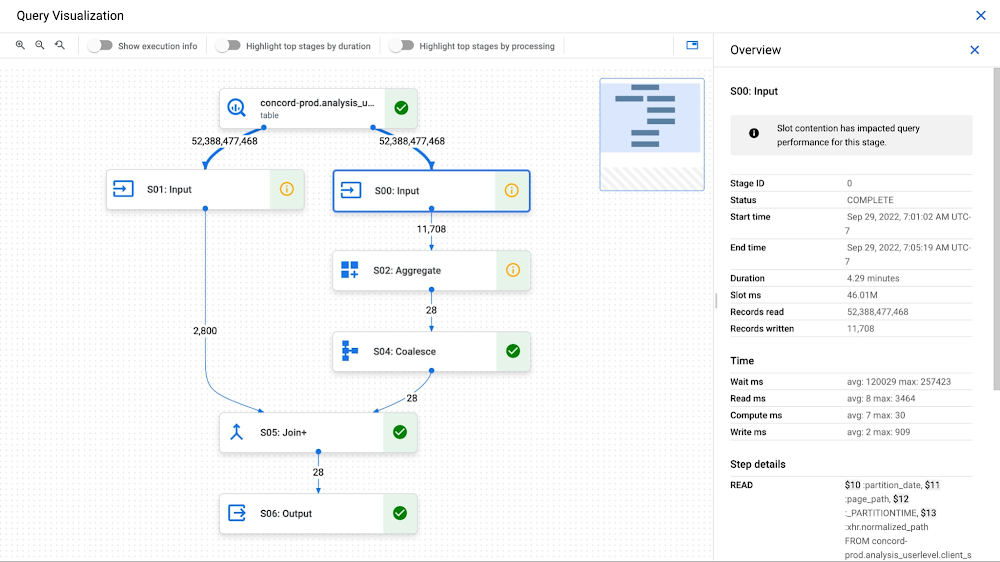
Execution graph
When BigQuery executes a query job, it converts the declarative SQL statement into a graph of execution, broken up into a series of query stages, which themselves are composed of more granular sets of execution steps. The query execution graph provides a visual representation of the execution stages and shows the corresponding metrics. Not all stages are made equal. Some are more expensive and time consuming than others. The execution graph provides toggles for highlighting critical stages, which makes it easier to spot the potential performance bottlenecks in the query.
Query performance insights
In addition to the detailed execution graph BigQuery also provides specific insights on possible factors that might be slowing query performance.
Slot contention
When you run a query, BigQuery attempts to break up the work needed by your query into tasks. A task is a single slice of data that is input into and output from a stage. A single slot picks up a task and executes that slice of data for the stage. Ideally, BigQuery slots execute tasks in parallel to achieve high performance. Slot contention occurs when your query has many tasks ready for slots to start executing, but BigQuery can’t get enough available slots to execute them.
Insufficient shuffle quota
Before running your query, BigQuery breaks up your query’s logic into stages. BigQuery slots execute the tasks for each stage. When a slot completes the execution of a stage’s tasks, it stores the intermediate results in shuffle. Subsequent stages in your query read data from shuffle to continue your query’s execution. Insufficient shuffle quota occurs when you have more data that needs to get written to shuffle than you have shuffle capacity.
Data input scale change
Getting this performance insight indicates that your query is reading at least 50% more data for a given input table than the last time you ran the query and hence experiencing query slowness. You can use table change history to see if the size of any of the tables used in the query has recently increased.
What’s next?
We continue to work on improving the visualization of the graph. We are working on adding additional metrics to each step and adding more performance insights that will make query diagnosis significantly easier. We are just getting started.
Research shows that over 90% of large organizations already deploy multicloud architectures, and their data is distributed across several public cloud providers. Additionally, data is also increasingly split across various storage systems such as warehouses, operational and relational databases, object stores, etc. With the proliferation of new applications, data is serving many more use cases such as data sciences, business intelligence, analytics, streaming and the list goes on. With these data trends, customers are increasingly gravitating towards an open multicloud data lake. However, multicloud data lakes present several challenges such as data silos, data duplication, fragmented governance, complexity of tools, and increased costs.
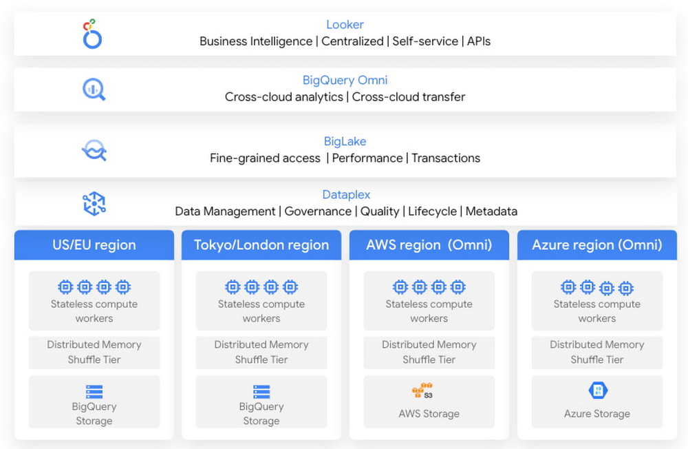
With Google’s data cloud technologies, customers can leverage the unique combination of distributed cloud services. They can create an agile cross-cloud semantic business layer with Looker and manage data lakes and data warehouses across cloud environments at scale with BigQuery and capabilities like BigLake and BigQuery Omni.
BigLake is a storage engine that unifies data warehouses and lake houses by standardizing across different storage formats including BigQuery managed table and open file formats such as Parquet and Apache Iceberg on object storage. BigQuery Omni provides the compute engine that runs locally to the storage on AWS or Azure, which customers can use to query data in AWS or Azure seamlessly. This provides several key benefits such as:
A single pane of glass to query your multicloud data lakes (across Google Cloud Platform, Amazon Web Services, and Microsoft Azure)
Cross-cloud analytics by combining data across different platforms with little to no egress costs
Unified governance and secure management of your data wherever it resides
In this blog, we will share cross-cloud analytics use cases customers are solving with Google’s Data Cloud and the benefits they are realizing.
Unified marketing analytics for 360-degree insights
Organizations want to perform marketing analytics – ads optimization, inventory management, churn prediction, buyer propensity trends and many more such analytics. To do this before BigQuery Omni, customers had to use data from several different sources such as Google Analytics, public datasets and other proprietary information stored across cloud environments. This requires moving large amounts of data, managing duplicate copies and incremental costs to perform any cross-cloud analytics and derive actionable insights. With BigQuery Omni, organizations are able to greatly simplify this workflow. Using the familiar BigQuery interface, users can access data residing in AWS or Azure, discover and select just the relevant data that needs to be combined for further analysis. This subset of data can be moved to Google Cloud using Omni’s new Cross-Cloud Transfer capabilities. Customers can combine this data with other Google Cloud datasets and these consolidated tables can be made available to key business stakeholders through advanced analytics tools such as Looker and Looker Studio. Customers are also able to tie in this data now with world class AI models via Vertex AI.
As an illustrative example, consider a retailer who has sales & inventory, user and search data spread across multiple data silos. Using BigQuery Omni they can seamlessly bring these datasets together and power several marketing analytics scenarios like customer segmentation, campaign management and demand forecasting etc.
“Interested in performing cross-cloud analytics, we tested BigQuery Omni and really liked the SQL support to easily get data from AWS S3. We have seen great potential and value in BigQuery Omni for adopting a multi-cloud data strategy.” — Florian Valeye, Staff Data Engineer,Back Market, a leading online marketplace for renewed technology based out of France
Data platform with consistent and unified cross-cloud governance
Another pattern is customers looking to analyze operational, transactional and business data across data silos in different clouds through a unified data platform. These data silos are a result of various factors such as merger and acquisitions, standardization of analytical tools, leveraging best of breed solutions in different clouds and diversification of data footprint across clouds. In addition to a single pane of glass for data access across silos, customers deeply desire consistent and uniform governance of their data across clouds.
With BigLake and BigQuery Omni abstracting the storage and compute layers respectively, organizations can access and query their data in Google Cloud irrespective of where it resides. They can also set fine-grained row level and column access policies in BigQuery and consistently govern it across clouds. These building blocks enable data engineering teams to build a unified and governed data platform for their data users without having to deal with the complexity of building and managing complex data pipelines. Furthermore, with BigQuery Omni’s integration with Dataplex and Data Catalog, you can discover, search your data across clouds and enrich your data by adding relevant business context with business glossary and rich text.
“Several SADA customers use GCP to build and manage their data analytics platform. During many explorations and proofs of concepts, our customers have seen the great potential and value in BigQuery Omni. Enabling seamless cross-cloud data analytics has allowed them to realize the value of their data quicker while lowering the barrier to entry for BigQuery adoption in a low-risk fashion.” — Brian Suk, Associate Chief Technology Officer,SADA, one of the strategic partners of Google Cloud.
Simplified data sharing between data providers and their customers
A third emerging pattern in cross cloud analytics is data sharing. Several services have the business need to share information such as inventory data, subscriber data to their customers or users who in turn analyze or aggregate the data with their proprietary data and oftentimes share the results back with the service provider. In several cases, the two parties are on different cloud environments, requiring them to move data back and forth.
Consider an example from a company Action IQ that operates in the customer data platform (CDP) space. CDPs were designed to help activate customer data, and a critical first step of that was unifying and managing that customer data. To enable this, many CDP vendors built their solution choosing one of the available cloud infrastructure technologies and copied data from the client’s systems. “Copying data from client applications and infrastructure has always been a requirement to deploy a CDP, but it doesn’t have to be anymore” — Justin DeBrabant, Senior Vice President of Product, ActionIQ.
While a small percentage of customers are fine with moving data across cloud environments, the majority are hesitant to onboard new services and would rather prefer providing governed access to their data sets.
“A new architectural pattern is emerging, allowing organizations to keep their data at one location and make it accessible, with the proper guardrails, to applications used by the rest of the organization’s stack”addsJustin at ActionIQ.
With BigQuery Omni, services in Google Cloud Platform can more easily access and share data with their customers and users in other cloud environments with limited data movement. One of UK’s largest statistics providers has explored Omni for their data sharing needs.
“We tested BigQuery Omni and really like the ability to get data from AWS directly into BQ. We’re excited about managing data sharing with different organizations without onboarding new clouds” – Simon Sandford-Taylor, Chief Information and Digital Officer, UK’s Office for National Statistics
With BigQuery Omni, customers are able to:
Access and query data across clouds through a single user interface
Reduce the need for data engineering before analyzing data
Lower operational overhead and risks by deploying an application that runs across multiple clouds which leverages the same, consistent security controls
Accelerate access to insights by significantly reducing the time for data processing and analysis
Create consistent and predictable budgeting across multiple cloud footprints
Enable long term agility and maximize the benefits every cloud investment
Over the last year, we’ve seen great momentum in customer adoption and added significant innovations to BigQuery Omni including improved performance and scalability for querying your data in AWS S3 or Azure Blob Storage, Iceberg support for Omni, Larger query result set size up to 10GB and Cross-cloud transfer that helps customers easily, securely, and cost effectively move just enough data across cloud environments for advanced analytics.
BigQuery Omni has launched several features to support unified governance of your data across multiple clouds – you can get fine-grained access to your multi-cloud data with row level and column level security. Building on this, we are excited to announce that BigQuery Omni now supports data masking. We’ve also made it easy for customers to try and see the benefits of BigQuery Omni through the limited time free trial available until March 30, 2023.
BigQuery Omni running on other public clouds outside of Google Cloud is available in AWS US East1 (N.Virginia) and Azure US East2 (US East) regions. We are also excited to share that we will be bringing BigQuery Omni to more regions in the future, starting with Asia Pacific (AWS Korea) coming soon.
Getting Started
Get started with a free trial to learn about Omni. Check out the documentation to learn more about BigQuery Omni. You can also leverage the self paced labs to learn how to set up BigQuery Omni easily.
Editor’s note: This post is part of an ongoing series on IT predictions from Google Cloud experts. Check out the full list of our predictions on how IT will change in the coming years.
Prediction: By 2025, 90% of data will be actionable in real-time using ML
A recent survey uncovered that only one-third of all companies are able to realize tangible value from their data. As a result, organizations are saddled with the operational burden of managing data infrastructure, moving and duplicating data, and making it available to the right users in the right tools.
In our own experience building data infrastructure, we’ve found the following principles to be helpful for overcoming barriers to value and innovation:
You have to be able to see and trust your data. First off, spend less time looking for your data. Then, leverage automation and intelligence to catalog your data so you can be sure that you can trust it. Using automatic cataloging tools like Dataplex allows you to discover, manage, monitor, and govern your data from one place, no matter where it’s stored. Instead of spending days searching for the right data, you can find it right when you need it and spend more time actually working with it. Plus, built-in data quality and lineage capabilities help automate data quality and troubleshoot data issues.
You have to be able to work with data. Adopt the best proprietary and open source tools that allow your teams to work across all of your data, from structured to semi-structured to unstructured. The key is finding ways to leverage the best of open source, like Apache Spark, while integrating enterprise solutions, so you can deliver reliability and performance at scale. Imagine what’s possible when you can leverage the power of Google Cloud infrastructure without forking the open source code?
You need to act on today’s data today — not tomorrow. Apply streaming analytics so you can work with data as it’s collected. Building unified batch and real-time pipelines allows you to process real-time events to achieve in-context experiences. For example, a streaming service like Dataflow lets you use Apache Beam to develop unified pipelines once and deploy in batch and real time.
When you can see the data, trust the data, and work with data as it’s collected, we can see how 90% of data will become actionable in real-time using ML and the incredible innovation that it will unlock.
In May 2022 at Google I/O, we announced the preview of AlloyDB for PostgreSQL, a fully-managed, PostgreSQL-compatible database service that provides a powerful option for modernizing your most demanding enterprise database workloads. We’re happy to announce that AlloyDB is now generally available.
AlloyDB is an excellent choice for organizations looking to break free from their legacy, proprietary databases and for existing PostgreSQL users looking to scale with no application changes. It combines full PostgreSQL compatibility with the best of Google: scale-out compute and storage, integrated analytics, and AI/ML-powered management. That means you get better performance, availability, and scalability with minimal management overhead.
Based on our performance tests, AlloyDB is more than four times faster for transactional workloads, and up to 100 times faster for analytical queries than standard PostgreSQL. It’s also two times faster for transactional workloads than Amazon’s comparable PostgreSQL-compatible service. You can expect high out-of-the-box regional availability, backed by a 99.99% availability SLA inclusive of maintenance. AlloyDB automatically detects and recovers from most database failures within 60 seconds, independent of database size and load. And finally, autopilot systems for automatic provisioning of storage, adaptive auto-vacuuming, and more make it easier than ever to manage your database. Pricing is transparent and predictable, with no expensive, proprietary licensing and no hidden I/O charges.
Since our preview announcement in May, we’ve introduced a number of new product capabilities to address the needs of high-end enterprise applications. We’ve added critical security features like customer-managed encryption keys (CMEK) and VPC Service Controls, and announced the preview of cross-region replication. We expanded configuration options, including introducing a new 2 vCPU /16 GB RAM machine type, and adding support for additional PostgreSQL extensions like pgRouting, PLV8, and amcheck. We continued to make AlloyDB easier to manage, introducing the preview of an index advisor and new fleet-wide monitoring.
Earlier, in September , we announced the preview of PostgreSQL to AlloyDB migrations with our easy-to-use, secure, and serverless Database Migration Service. We also announced the preview of AlloyDB’s integration with Datastream for seamless change data capture and replication to destinations like BigQuery. And finally, we continued to make improvements in performance, availability, replication lag, and monitoring to better meet the needs of your workloads.
Customer and partner momentum
We’re seeing increased momentum from organizations looking to modernize their database estates with high performance, scale, and availability. At this opportunity we’d like to thank everyone who participated in the preview and sent us useful feedback.
B4A, a Brazilian beauty-tech startup, is one such customer. B4A was founded with the purpose of democratizing the beauty market, offering monthly beauty subscription services to more than 100,000 paying subscribers. “We opted for AlloyDB for performance reasons, and indeed, the results were amazing,” says Jan Riehle, CEO and Founder at B4A. “Combining AlloyDB with a GraphQL API decreased query times for our full catalog of products by up to 90 percent compared to our previous database solution. We also came to appreciate the ease of maintenance that a fully managed solution like AlloyDB provides – setting up and configuring the database was a very smooth process that went really quickly for us. And compared to our previous database, we’ve been able to cut costs, and are no longer stuck paying for traditional database licenses.”
London-based technology company Thought Machine is on a mission to create technology that can run the world’s banks according to the best designs and software practices of the modern age. “We were delighted to be in the preview programme with AlloyDB, and now to be a launch partner as it comes into general availability,” says Will Montgomery, CTO at Thought Machine. “We are confident that AlloyDB performs at the highest level for our global Tier 1 bank clients running on Google Cloud Platform, which have stringent demands on performance and availability.”
Today we’re also happy to announce the expansion of the AlloyDB partner ecosystem with several new partnerships, for a total of over 50 technology and service partners to support your AlloyDB-based deployments. Technology vendors are ready to support your needs in business intelligence, advanced analytics, data integration, governance, observability, and migration assessment, while regional and global service partners have the necessary expertise to help your database migrations and other implementation needs. Read more about the expanded AlloyDB partner ecosystem.
What else do I need to know?
Preview pricing will continue through December 31, 2023, after which normal billing will commence. For additional pricing information, see AlloyDB pricing. You can find more information about product functionality, regional availability, and our service-level agreement (SLA) in the AlloyDB for PostgreSQL documentation.
Learn more about AlloyDB
Check out the Introducing AlloyDB for PostgreSQL video for the full story on migrating, modernizing and building applications with AlloyDB. You can also learn about the technology underlying AlloyDB from our “Under the Hood” blog series. We cover the disaggregation of compute and storage in Intelligent, database-aware storage and explore AlloyDB’s vectorized columnar execution engine, which enables analytical acceleration with no impact on operational performance, in the Columnar engine blog post.
Also check our animated video series, “Introducing AlloyDB”. The first episode, What is AlloyDB?, discusses how AlloyDB provides full PostgreSQL compatibility together with accelerated database performance, high availability, and analytics integration. Be sure to subscribe for future episodes.
What is AlloyDB? The first episode in the animated series, “Introducing AlloyDB”.
Getting started
You can get started with AlloyDB in just a few clicks by navigating to the AlloyDB console and creating your first cluster.
Getting started is easy with three simple steps:
Create your AlloyDB cluster
Create a primary instance for that cluster
Connect to the cluster using a psql client
Check out our quickstart for a step-by-step guide on creating a new AlloyDB cluster. Or you can use Database Migration Service to easily migrate an existing PostgreSQL database to AlloyDB.