Blog

Monitoring machine learning (ML) models in production is now as simple as using a function in BigQuery! Today we’re introducing a new set of functions that enable model monitoring directly within BigQuery. Now, you can describe data throughout the model workflow by profiling training or inference data, monitor skew between training and serving data, and monitor drift in serving data over time using SQL — for BigQuery ML models as well as any model whose feature training and serving data is available through BigQuery. With these new functions, you can ensure your production models continue to deliver value while simplifying their monitoring.

In this blog, we present two companion notebooks to help you get hands-on with these features today!

Companion Introduction – a fast introduction to all the new functions

Companion Tutorial – an in-depth tutorial covering many usage patterns for the new functions, including using Vertex AI Endpoints, monitoring feature attributions, and an overview of how monitoring metrics are calculated.

The foundation of a model: the data

A model is only as good as the data it learns from. Understanding the data deeply is essential for effective feature engineering, model selection, and ensuring quality through MLOps. BigQuery’s table-valued function ML.DESCRIBE_DATA provides a powerful tool for this, allowing you to summarize and describe an entire table with a single query.

Example: Identifying data issues

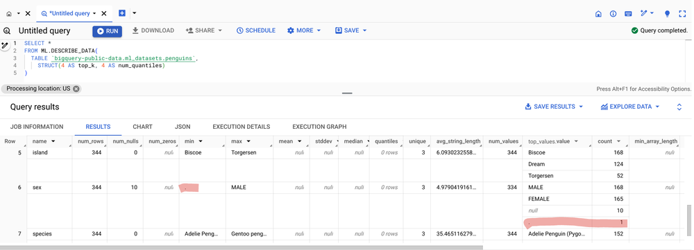
In the accompanying introduction notebook, we profile the training data ( penguin classification dataset) using   the ML.DESCRIBE DATA  function and quickly identify a data issue.

Here’s the resulting output table:

Notice that the min value for the sex column is a ‘.’. Ideally, we’d see the values MALE, FEMALE or null as indicated in the top_values.values column. This means that in addition to the 10 null values (indicated by the num_null column) there are also some null values indicated by a string with value ‘.’. This should be corrected before using it as training data. 

The ML.DESCRIBE_DATA function is extra helpful because it summarizes each data type all in one table. There are also optional parameters that can be specified to control the number of quantiles for different numerical column types and the number of top values to return for categorical columns. The input data can be specified as a table or a query statement, allowing you to describe specific subsets of data (e.g., serving timeframes, or groups within your training data). The function’s flexibility extends beyond ML tasks: it even allows you to describe data stored outside of BigQuery, facilitating quick analysis for both model-building and broader data exploration purposes.

Detect skew at a glance

A trained model will perform only when the serving data is similar in distribution to the training data. Model monitoring helps ensure this by comparing training and serving data for shifts known as skew. BigQuery’s ML.VALIDATE_DATA_SKEW table valued function streamlines this process, allowing you to directly compare serving data to any BigQuery ML model’s training data.

Let’s see it in action:

This query directly compares the data in the serving table to the BigQuery ML model classify_species_logistic. The accompanying introduction notebook has the full code in an interactive example. In that notebook the serving data is simulated to create change in two of the features: body_mass_g and flipper_length_mm. The results of the ML.VALIDATE_SKEW function show anomalies detect for each of these:

The detection of skew is as easy as comparing a model in BigQuery to a table of serving data. During training, BigQuery ML models automatically compute and store relevant statistics. This eliminates the need for reusing the entire training dataset, making skew monitoring simple and cost-efficient. Importantly, the function intelligently focuses on features present in the model, further enhancing efficiency and workflow. With optional parameters, you can customize anomaly detection thresholds, metric types for categorical features, and even set different thresholds for specific features. Later, we’ll demonstrate how easily you can monitor skew for any model!

Proactive monitoring for drift

Beyond comparing serving data to training data, it’s also important to keep an eye on changes within serving data over time. Comparing recent serving data to previous serving data is another type of model monitoring known as drift detection. This uses the same detection techniques of metrics that compare distributions between a baseline and comparison dataset and flag anomalies that exceed set threshold. With the table valued function ML.VALIDATE_DATA_DRIFT, you can compare any two tables, or query statements results, directly for detection. 

Drift detection in action:

Here, the same serving table is used as the baseline and comparison table but with different WHERE statements to filter the rows and compare today to yesterday as an example. The results below show that while the detection values did not surpass the threshold, they are approaching the threshold between two consecutive days for the features that have simulated change.

Just like with skew detection, you can also adjust the default detection threshold for anomaly detection as well as the metric type used for categorical features, and specify different thresholds for different columns and feature types. There are additional parameters to control the binning of numerical features for the metrics calculations. 

Take TFDV monitoring to the next level

If you’re already familiar with the TensorFlow Data Validation (TFDV) library, you’ll appreciate how these new BigQuery functions enhance your model monitoring toolkit. They bring the power of TFDV directly into your BigQuery workflows, allowing you to generate rich statistics, detect anomalies, and leverage TFDV’s powerful visualization tools — all with SQL. And the best part is it uses BigQuery’s scalable, serverless compute. Leverage BigQuery’s scalable, serverless compute for near-instant analysis, empowering you to take rapid action on model monitoring insights!

Let’s explore how it works:

Generate statistics with ML.TFDV_DESCRIBE

You can generate in-depth statistics summaries with table valued function ML.TFDV_DESCRIBE for any table, or query, in the same format as the TensorFlow tfdv.generate_statistics_from_csv() API:

The ML.TFDV_DESCRIBE function outputs statistics in a structured data format (a ‘proto’) that is directly compatible with TFDV: tfmd.proto.statistics_pb2.DatasetFeatureStatisticsList. 

Using a bit of Python code in a BigQuery notebook, we can import the TFDV package as well as TensorFlow Metadata package and then make a call to the tfdv.visualize_statistics method while converting the data to the expected format. The ML.TFDV_DESCRIBE results were loaded to Python for the training data as train_describe and for the current day’s serving data as today_describe. See the accompanying tutorial for complete details.

This generates the amazing visualizations shown below that directly highlight shifts in the two parameters that we purposefully shifted in the serving data for this example: body_mass_g and flipper_length_mm

This streamlined workflow brings the power and precision of TensorFlow Data Validation directly to BigQuery and enables you to quickly visualize how sets of data differ. This provides deeper insight to model health monitoring and informs how to proceed with model training iterations.

Detect anomalies With ML.TFDV_VALIDATE

You can also precisely detect skew or drift anomalies with the scalar function ML.TFDV_VALIDATE, which compares tables, or queries, pinpointing potential model-breaking shifts.

Example:

These results are formatted in a structured data format (‘proto’) that is specifically compatible with TFDV’s display tools: tfmd.proto.anomalies_pbs2.Anomalies. Passing this as input to Python method tfdv.display_anomalies presents an easy-to-read table of anomaly detection results as presented after the code snippet:

The default detection methods for numerical and categorical data, as well as thresholds are the same as for the other functions shown above. You can customize detection with parameters in the function for precision monitoring needs. For a deeper dive, the accompanying tutorial includes a section that demonstrates how these metrics are calculated manually and uses this function to compare to the manual calculation results as a validation.

Online and batch serving: A unified model monitoring approach

BigQuery’s model monitoring functions offer a streamlined solution whether you’re working with models deployed on Vertex AI Prediction Endpoints or using batch serving data stored within BigQuery (as shown above). Here’s how:

Batch serving: For batch prediction data already stored or accessible by BigQuery, the monitoring features are readily accessible just as demonstrated previously in this blog.

Online serving: Directly monitor models deployed on Vertex AI Prediction Endpoints. By configuring logging requests and responses to BigQuery, you can easily apply BigQuery ML model monitoring functions to detect skew and drift. 

The accompanying tutorial provides a step-by-step walkthrough, demonstrating endpoint creation, model deployment, logging setup (for Vertex AI to BigQuery), and how to monitor both online and batch serving data within BigQuery.

Automate for scale

To achieve truly scalable monitoring of shifts and drifts, automation is essential. BigQuery’s procedural language offers a powerful way to streamline this process, as demonstrated in the SQL query from our introductory notebook. This automation isn’t limited to monitoring; it can extend to continuous model retraining. In a production environment, continuous training would be accompanied by: proactively identifying data quality issues, adapting to real-world changes, and maintaining a rigorous deployment strategy aligned with your organization’s needs.

Let’s take a look at what the results look like:

A skew anomaly was detected and successfully triggered model retraining, restoring accuracy after the data changes. This demonstrates the value of automated monitoring and retraining for maintaining model performance in dynamic production environments.

To streamline this process, Google Cloud offers several powerful automation options::

BigQuery Scheduled Queries

Dataform

Workflows

Cloud Composer

Vertex AI Pipelines

Want a hands-on demonstration? Our accompanying tutorial dives into BigQuery scheduled queries, including historical backfilling, daily monitoring, and setting up email alerts for detected shifts and drifts. We’ll also be releasing future tutorials covering the other automation tools.

The simplicity and power of model monitoring With BigQuery

Building trustworthy machine learning systems requires continuous monitoring. BigQuery’s new model monitoring functions streamline this to just a few SQL functions:

Deeply understand your data: ML.DESCRIBE_DATA provides a comprehensive view of your datasets, aiding in feature engineering and quality checks.

Detect skew between training and serving data: ML.VALIDATE_DATA_SKEW directly compares BigQuery ML models against their serving data.

Monitor data drift over time: ML.VALIDATE_DATA_DRIFT empowers you to track changes in serving data, ensuring your model’s performance remains consistent.

Enhance your TFDV workflow: ML.TFDV_DESCRIBE and ML.TFDV_VALIDATE bring the precision of TensorFlow Data Validation directly into BigQuery, enabling more detailed visualizations and anomaly detection while leveraging BigQuery’s scalable, and efficient compute.

Getting Started

Extend from BigQuery ML models to Vertex AI Models and automate these new functions with Google Cloud offerings like BigQuery scheduled queries, Dataform, Workflows, Cloud Composer, or Vertex AI Pipelines. Dive into our hands-on notebooks to get started today:

Companion Introduction – a fast introduction to all the new functions

Companion Tutorial – an in-depth tutorial covering many usage patterns for the new functions, including using Vertex AI Endpoints, monitoring feature attributions, and an overview of how monitoring metrics are calculated

In today’s AI era, data is your competitive edge.

There has never been a more exciting time in technology, with AI creating entirely new ways to solve problems, engage customers, and work more efficiently. 

However, most enterprises still struggle with siloed data, which stifles innovation, keeps vital insights locked away, and can reduce the value AI has across the business. 

Discover a faster, smarter way to innovate

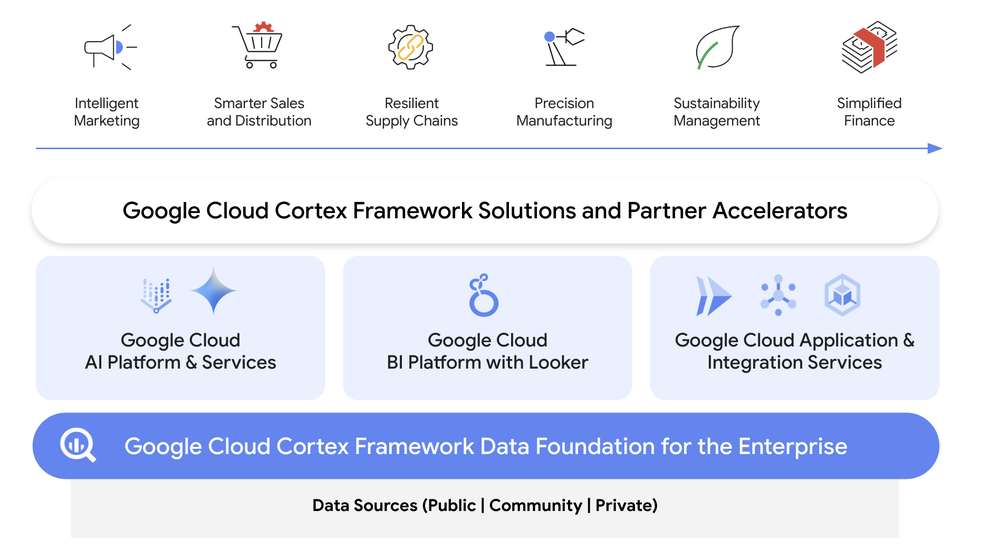
Google Cloud Cortex Framework accelerates your ability to unify enterprise data for connected insights, and provides new opportunities for AI to transform customer experiences, boost revenue, and reduce costs which can otherwise be hidden in your company’s data and applications. 

Built on an AI-ready Data Cloud foundation, Cortex Framework includes what you need to design, build, and deploy solutions for specific business problems and opportunities including endorsed reference architectures and packaged business solution deployment content. In this blog, we provide an overview of Cortex Framework, and highlight some recent enhancements.

Get a connected view of your business with one data foundation 

Cortex Framework enables one data foundation for businesses by bridging and enriching private, public, and community insights for deeper analysis.

Our latest release extends Cortex Data Foundation with new data and AI solutions for enterprise data sources including Salesforce Marketing Cloud, Meta, SAP ERP, and Dun & Bradstreet. Together this data unlocks insights across the enterprise and opens up opportunities for optimization and innovation. 

New intelligent marketing use cases

Drive more intelligent marketing strategies with one data foundation for your enterprise data, including integrated sources like Google Ads, Campaign Manager 360, TikTok and now — Salesforce Marketing Cloud and Meta connectivity with BigQuery via Cortex Framework, with predefined data ingestion templates, data models and sample dashboards. Together with other business data available like sales and supply chain sources in Cortex Data Foundation, you can accelerate insights and answer questions like: How does my overall campaign and audience performance relate to sales and supply chain?

New sustainability management use cases

Want more timely insights into environment, social and governance (ESG) risks and opportunities? You can now manage ESG performance and goals with new vendor ESG performance insights using Dun & Bradstreet ESG ranking data connected with your SAP ERP supplier data. Now with predefined data ingestion templates, data models and a sample dashboard focused on sustainability insights, for informed decision making. Answer questions like: “What is my raw material suppliers’ ESG performance against industry peers?” “What is their ability to measure and manage GHG emissions?” and “What is their adherence and commitment to environmental compliance and corporate governance?”

New simplified finance use cases

Simplify financial insights across the business to make informed decisions about liquidity, solvency, and financial flexibility to feed into strategic growth investment opportunities — now with predefined data ingestion templates, data models and sample dashboards to help you discern new insights with balance sheet and income statement reporting on SAP ERP data.

Accelerate AI innovation with secured data access

To help organizations build out a data mesh for more optimized data discovery, access control and governance when interacting with Cortex Data Foundation, our new solution content offers a metadata framework built on BigQuery and Dataplex that:

Organizes Cortex Data Foundation pre-defined data models into business domains

Augments Cortex Data Foundation tables, views and columns with semantic context to empower search and discovery of data assets

Enables natural language to SQL capabilities by providing logical context for Cortex Data Foundation content to LLMs and gen AI applications

Annotates data access policies to enable consistent enforcement of access controls and masking of sensitive columns

With a data mesh in place, Cortex Data Foundation models can allow for more efficiency in generative AI search and discovery, as well as fine-grained access policies and governance. 

Data and AI brings next-level innovation and efficiency 

Will your business lead the way? Learn more about our portfolio of solutions by tuning in to our latest Next ‘24 session – ANA107 and checking out our website.