Google Cloud CLI makes it very quick and easy for engineers to get started with initial development on Google Cloud Platform and perform many common cloud tasks. The majority of the initial development experience is via the command line interface using tools like gsutil, gcloud, but getting the code to production requires writing ceremonial code or building API-level integration.
Developers often come across scenarios where they need to run simple commands in their production environment on a scheduled basis. In order to execute on this successfully, they are required to code and create schedules in an orchestration tool such as Data Fusion or Cloud Composer.
One such scenario is copying objects from one bucket to another (e.g. GCS to GCS or S3 to GCS), which is generally achieved by using gsutil. Gsutil is a Python application that is used to interact with Google Cloud Storage through the command line. It can be used to perform a wide range of functions such as bucket and object management tasks, including: creating and deleting buckets, uploading, downloading, deleting, copying and moving objects.
In this post, we will describe an elegant and efficient way to schedule commands like Gsutil using Cloud Run and Cloud Scheduler. This methodology saves time and reduces the amount of effort required for pre-work and setup in building API level integration.
You can find the complete source code for this solution within our Github.
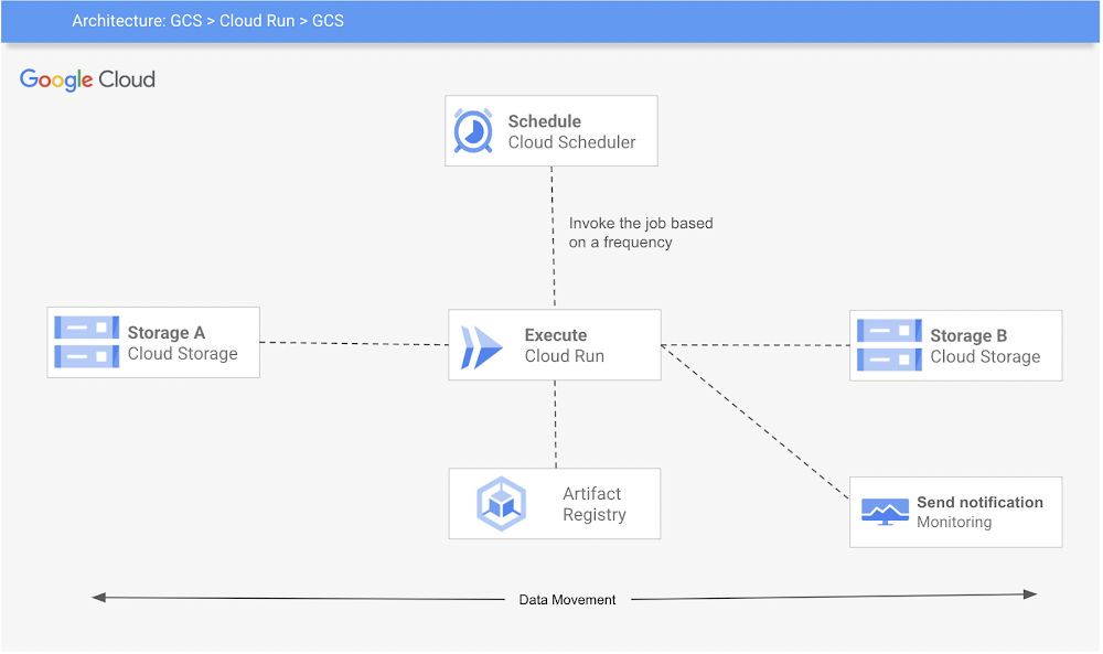
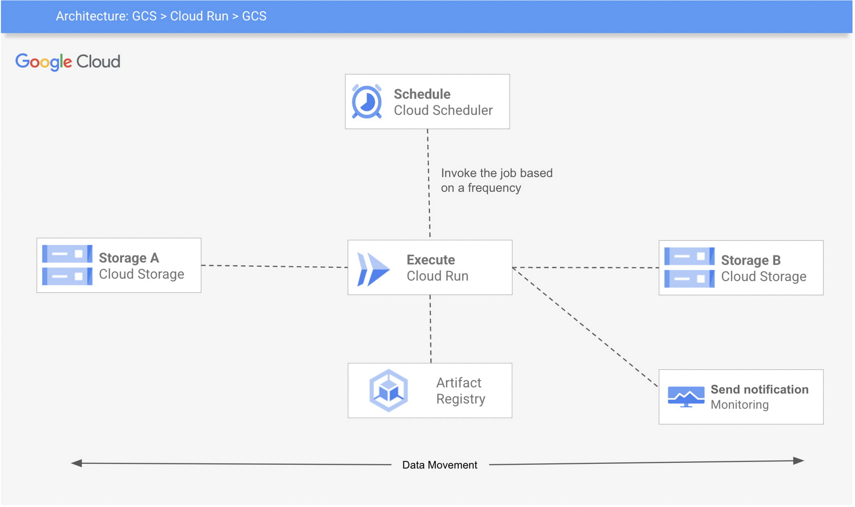
Here’s a look at the architecture of this process:
The 3 Google Cloud Platform (GCP) services used are:
Cloud Run: The code will be wrapped in a container, gcloud SDK will be installed ( or you can also use a base image with gcloud SDK already installed). Cloud Scheduler: A Cloud Scheduler job invokes the job created in Cloud Run on a recurring schedule or frequency.Cloud Storage: Google Cloud Storage (GCS) is used for storage and retrieval of any amount of data.
This example requires you to set up your environment for Cloud Run and Cloud Scheduler, create a Cloud Run job, package it into a container image, upload the container image to Container Registry, and then deploy to Cloud Run. You can also build monitoring for the job and create alerts. Follow below steps to achieve that:
Step 1: Enable services (Cloud Scheduler, Cloud Run) and create a service account
code_block[StructValue([(u’code’, u’export REGION=<<Region>>rnexport PROJECT_ID=<<project-id>>rnexport PROJECT_NUMBER=<<project-number>>rnexport SERVICE_ACCOUNT=cloud-run-sarnrngcloud services enable cloudscheduler.googleapis.com run.googleapis.com cloudbuild.googleapis.com cloudscheduler.googleapis.com –project ${PROJECT_ID}rnrngcloud iam service-accounts create ${SERVICE_ACCOUNT} \rn –description=”Cloud run to copy cloud storage objects between buckets” \rn –display-name=”${SERVICE_ACCOUNT}” –project ${PROJECT_ID}rnrngcloud projects add-iam-policy-binding ${PROJECT_ID} \rn –member serviceAccount:${SERVICE_ACCOUNT}@${PROJECT_ID}.iam.gserviceaccount.com \rn –role “roles/run.invoker”‘), (u’language’, u”), (u’caption’, <wagtail.wagtailcore.rich_text.RichText object at 0x3e20a44c5f10>)])]
To deploy a Cloud Run service using a user-managed service account, you must have permission to impersonate (iam.serviceAccounts.actAs) that service account. This permission can be granted via the roles/iam.serviceAccountUser IAM role.
Step 3: Create a job with the GCS_SOURCE and GCS_DESTINATION for gcs-to-gcs bucket. Make sure to give the permission (roles/storage.legacyObjectReader) to the GCS_SOURCE and roles/storage.legacyBucketWriter to GCS_DESTINATION
code_block[StructValue([(u’code’, u’export GCS_SOURCE=<<Source Bucket>>rnexport GCS_DESTINATION=<<Source Bucket>>rnrngsutil iam ch \rnserviceAccount:${SERVICE_ACCOUNT}@${PROJECT_ID}.iam.gserviceaccount.com:objectViewer \rn ${GCS_SOURCE}rnrngsutil iam ch \rnserviceAccount:${SERVICE_ACCOUNT}@${PROJECT_ID}.iam.gserviceaccount.com:legacyBucketWriter \rn ${GCS_DESTINATION}rnrngcloud beta run jobs create gcs-to-gcs \rn –image gcr.io/${PROJECT_ID}/gsutil-gcs-to-gcs \rn –set-env-vars GCS_SOURCE=${GCS_SOURCE} \rn –set-env-vars GCS_DESTINATION=${GCS_DESTINATION} \rn –max-retries 5 \rn –service-account ${SERVICE_ACCOUNT}@${PROJECT_ID}.iam.gserviceaccount.com \rn –region $REGION –project ${PROJECT_ID}’), (u’language’, u”), (u’caption’, <wagtail.wagtailcore.rich_text.RichText object at 0x3e20a44c5310>)])]
Step 4: Finally, create a schedule to run the job.
Step 5: Create monitoring and alerting to check if the cloud run failed.
Cloud Run is automatically integrated with Cloud Monitoring with no setup or configuration required. This means that metrics of your Cloud Run services are captured automatically when they are running.
You can view metrics either in Cloud Monitoring or in the Cloud Run page in the console. Cloud Monitoring provides more charting and filtering options. Follow these steps to create and view metrics on Cloud Run.
The steps described in the blog present a simplified method to invoke the most commonly used developer-friendly CLI commands on a schedule, in a production setup. The code and example provided above are easy to use and help avoid the need of API level integration to schedule commands like gsutil, gcloud etc.
Iteration and innovation fuel the data-driven culture at Mercado Libre. In our first post, we presented our continuous intelligence approach, which leverages BigQuery and Looker to create a data ecosystem on which people can build their own models and processes.
Using this framework, the Shipping Operations team was able to build a new solution that provided near real-time data monitoring and analytics for our transportation network and enabled data analysts to create, embed, and deliver valuable insights.
The challenge
Shipping operations are critical to success in e-commerce, and Mercado Libre’s process is very complex since our organization spans multiple countries, time zones, and warehouses, and includes both internal and external carriers. In addition, the onset of the pandemic drove exponential order growth, which increased pressure on our shipping team to deliver more while still meeting the 48-hour delivery timelines that customers have come to expect.
This increased demand led to the expansion of fulfillment centers and cross-docking centers, doubling and tripling the nodes of our network (a.k.a. meli-net) in the leading countries where we operate. We also now have the largest electric vehicle fleet in Latin America and operate domestic flights in Brazil and Mexico.
We previously worked with data coming in from multiple sources, and we used APIs to bring it into different platforms based on the use case. For real-time data consumption and monitoring, we had Kibana, while historical data for business analysis was piped into Teradata. Consequently, the real-time Kibana data and the historical data in Teradata were growing in parallel, without working together. On one hand, we had the operations team using real-time streams of data for monitoring, while on the other, business analysts were building visualizations based on the historical data in our data warehouse.
This approach resulted in a number of problems:
The operations team lacked visibility and required support to build their visualizations. Specialized BI teams became bottlenecks.
Maintenance was needed, which led to system downtime.
Parallel solutions were ungoverned (the ops team used an Elastic database to store and work with attributes and metrics) with unfriendly backups and data bounded for a period of time.
We couldn’t relate data entities as we do with SQL.
Striking a balance: real-time vs. historical data
We needed to be able to seamlessly navigate between real-time and historical data. To address this need, we decided to migrate the data to BigQuery, knowing we would leverage many use cases at once with Google Cloud.
Once we had our real-time and historical data consolidated within BigQuery, we had the power to make choices about which datasets needed to be made available in near real-time and which didn’t. We evaluated the use of analytics with different time windows tables from the data streams instead of the real-time logs visualization approach. This enabled us to serve near real-time and historical data utilizing the same origin.
We then modeled the data using LookML, Looker’s reusable modeling language based on SQL, and consumed the data through Looker dashboards and Explores. Because Looker queries the database directly, our reporting mirrored the near real-time data stored in BigQuery. Finally, in order to balance near real-time availability with overall consumption costs, we analyzed key use cases on a case-by-case basis to optimize our resource usage.
This solution prevented us from having to maintain two different tools and featured a more scalable architecture. Thanks to the services of GCP and the use of BigQuery, we were able to design a robust data architecture that ensures the availability of data in near real-time.
Streaming data with our own Data Producer Model: from APIs to BigQuery
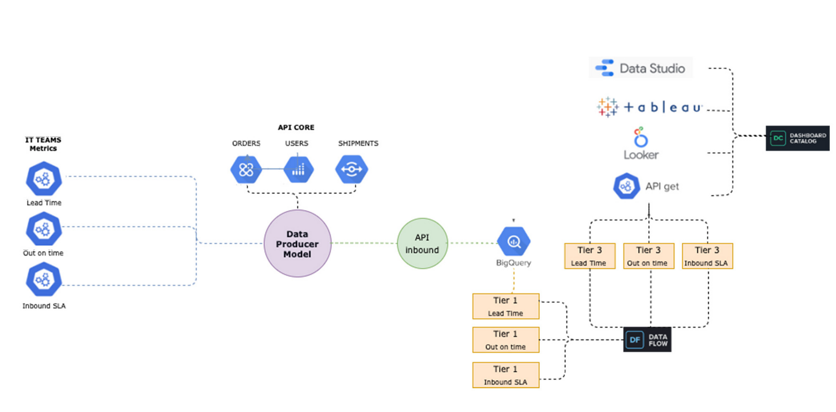
To make new data streams available, we designed a process which we call the “Data Producer Model” (“Modelo Productor de Datos” or MPD) where functional business teams can serve as data creators in charge of generating data streams and publishing them as related information assets we call “data domains”. Using this process, the new data comes in via JSON format, which is streamed into BigQuery. We then use a 3-tiered transformation process to convert that JSON into a partitioned, columnar structure.
To make these new data sets available in Looker for exploration, we developed a Java utility app to accelerate the development of LookML and make it even more fun for developers to create pipelines.
The end-to-end architecture of our Data Producer Model.
The complete “MPD” solution results in different entities being created in BigQuery with minimal manual intervention. Using this process, we have been able to automate the following:
The creation of partitioned, columnar tables in BigQuery from JSON samples
The creation of authorized views in a different GCP BigQuery project (for governance purposes)
LookML code generation for Looker views
Job orchestration in a chosen time window
By using this code-based incremental approach with LookML, we were able to incorporate techniques that are traditionally used in DevOps for software development, such as using Lams to validate LookML syntax as a part of the CI process and testing all our definitions and data with Spectacles before they hit production. Applying these principles to our data and business intelligence pipelines has strengthened our continuous intelligence ecosystem. Enabling exploration of that data through Looker and empowering users to easily build their own visualizations has helped us to better engage with stakeholders across the business.
The new data architecture and processes that we have implemented have enabled us to keep up with the growing and ever-changing data from our continuously expanding shipping operations. We have been able to empower a variety of teams to seamlessly develop solutions and manage third party technologies, ensuring that we always know what’s happening – and more critically – enabling us to react in a timely manner when needed.
Outcomes from improving shipping operations:
Today, data is being used to support decision-making in key processes, including:
Carrier Capacity Optimization
Outbound Monitoring
Air Capacity Monitoring
This data-driven approach helps us to better serve you -and everyone- who expects to receive their packages on-time according to our delivery promise. We can proudly say that we have improved both our coverage and speed, delivering 79% of our shipments in less than 48 hours in the first quarter of 2022.
Here is a sneak peek into the data assets that we use to support our day-to-day decision making:
a. Carrier Capacity: Allows us to monitor the percentage of network capacity utilized across every delivery zone and identify where delivery targets are at risk in almost real time.
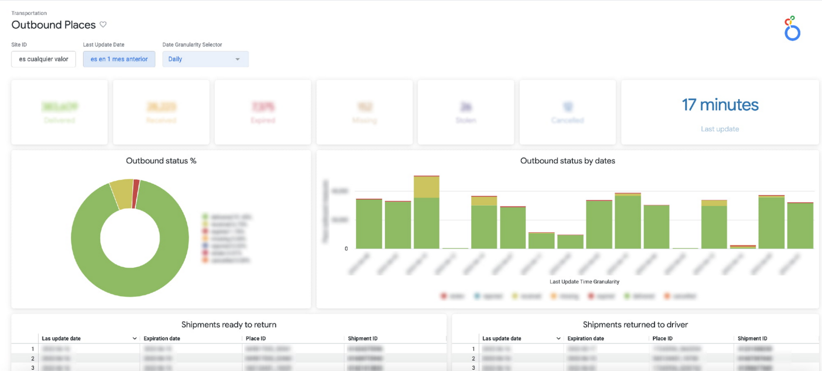
b. Outbound Places Monitoring: Consolidates the number of shipments that are destined for a place (the physical points where a seller picks up a package), enabling us to both identify places with lower delivery efficiency and drill into the status of individual shipments.
c. The Air Capacity Monitoring: Provides capacity usage monitoring for our aircrafts running each of our shipping routes.
Costs into the equation
The combination of BigQuery and Looker also showed us something we hadn’t seen before: overall cost and performance of the system. Traditionally, developers maintained focus on metrics like reliability and uptime without factoring in associated costs.
By using BigQuery’s information schema, Looker Blocks, and the export of BigQuery logs, we have been able to closely track data consumption, quickly detect underperforming SQL and errors, and make adjustments to optimize our usage and spend.
Based on that, we know the Looker Shipping Ops dashboards generate a concurrency of more than 150 queries, which we have been able to optimize by taking advantage of BigQuery and Looker caching policies.
The challenges ahead
Using BigQuery and Looker has enabled us to solve numerous data availability and data governance challenges: single point access to near real-time data and to historical information, self-service analytics & exploration for operations and stakeholders across different countries & time zones, horizontal scalability (with no maintenance), and guaranteed reliability and uptime (while accounting for costs), among other benefits.
However, in addition to having the right technology stack and processes in place, we also need to enable every user to make decisions using this governed, trusted data. To continue achieving our business goals, we need to democratize access not just to the data but also to the definitions that give the data meaning. This means incorporating our data definitions with our internal data catalog and serving our LookML definitions to other data visualizations tools like Data Studio, Tableau or even Google Sheets and Slides so that users can work with this data through whatever tools they feel most comfortable using.
If you would like a more indepth look at how we made new data streams available from a process we designed called the “Data Producer Model” (“Modelo Productor de Datos” or MPD) register to attend our webcast on August 31.
While learning and adopting new technologies can be a challenge, we are excited to tackle this next phase, and we expect our users will be too, thanks to a curious and entrepreneurial culture. Are our teams ready to face new changes? Are they able to roll out new processes and designs? We’ll go deep on this in our next post.
The cybersecurity industry is faced with the tremendous challenge of analyzing growing volumes of security data in a dynamic threat landscape with evolving adversary behaviors. Today’s security data is heterogeneous, including logs and alerts, and often comes from more than one cloud platform. In order to better analyze that data, we’re excited to announce the release of the Cloud Analytics project by the MITRE Engenuity Center for Threat-Informed Defense, and sponsored by Google Cloud and several other industry collaborators.
Since 2021, Google Cloud has partnered with the Center to help level the playing field for everyone in the cybersecurity community by developing open-source security analytics. Earlier this year, we introduced Community Security Analytics (CSA) in collaboration with the Center to provide pre-built and customizable queries to help detect threats to your workloads and to audit your cloud usage. The Cloud Analytics project is designed to complement CSA.
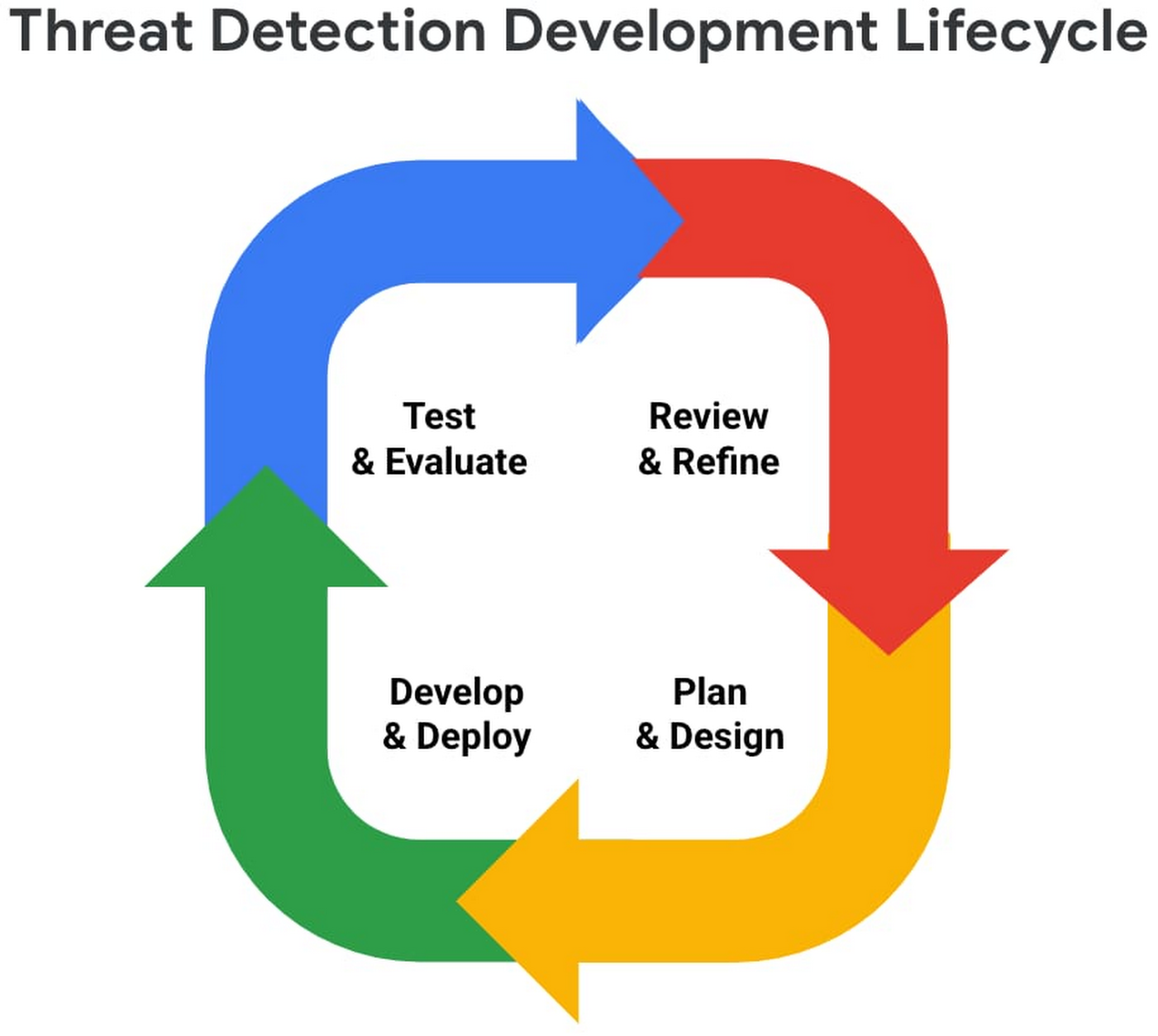
The Cloud Analytics project includes a foundational set of detection analytics for key tactics, techniques and procedures (TTPs) implemented as vendor-agnostic Sigma rules, along with their adversary emulation plans implemented with CALDERA framework. Here’s a overview of Cloud Analytics project, how it complements Google Cloud’s CSA to benefit threat hunters, and how they both embrace Autonomic Security Operations principles like automation and toil reduction (adopted from SRE) in order to advance the state of threat detection development and continuous detection and response (CD/CR).
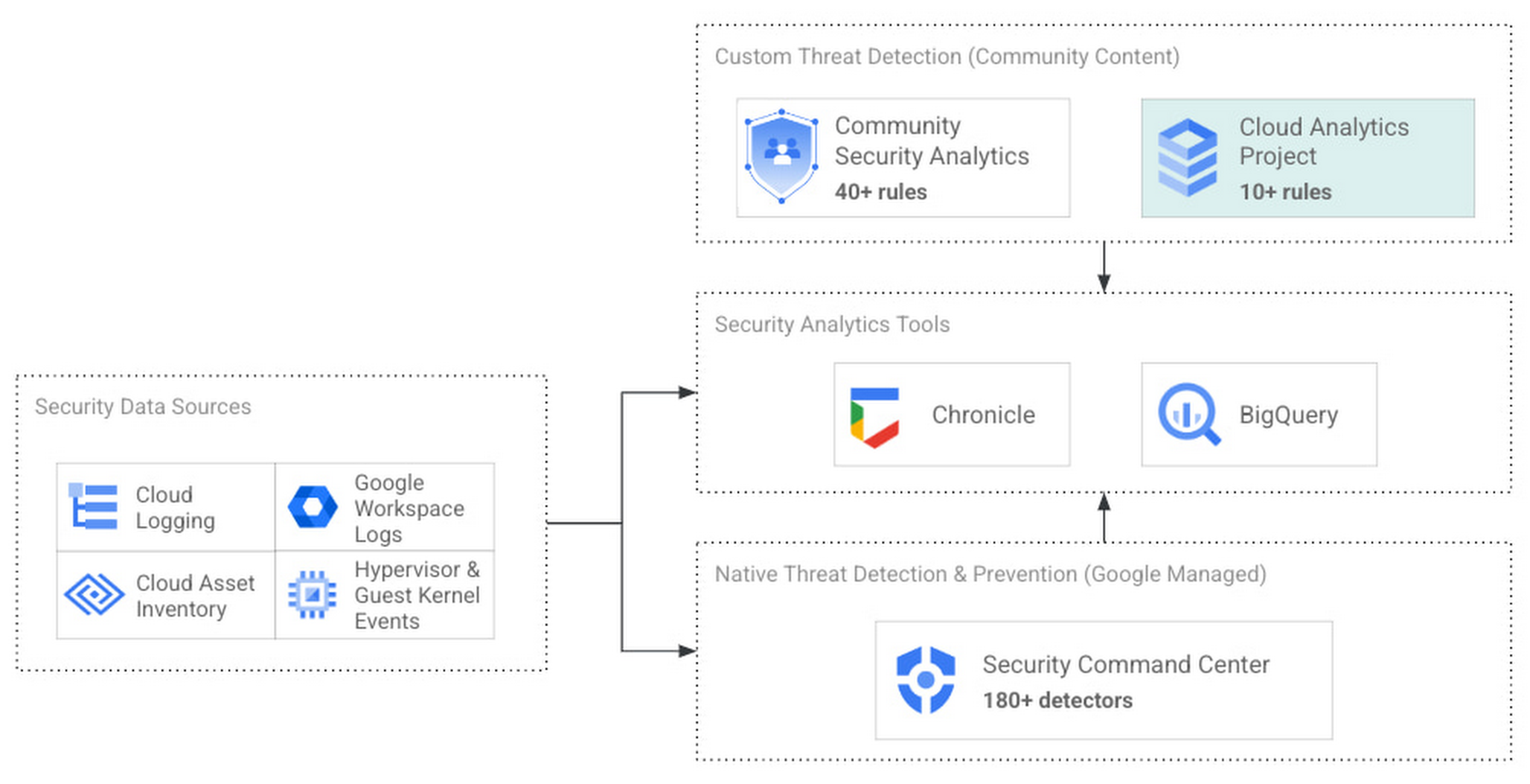
Both CSA and the Cloud Analytics project are community-driven security analytics resources. You can customize and extend the provided queries, but they take a more do-it-yourself approach—you’re expected to regularly evaluate and tune them to fit your own requirements in terms of threat detection sensitivity and accuracy. For managed threat detection and prevention, check out Security Command Center Premium’s realtime and continuously updated threat detection services including Event Threat Detection, Container Threat Detection, and Virtual Machine Threat Detection. Security Command Center Premium also provides managed misconfiguration and vulnerability detection with Security Health Analytics and Web Security Scanner.
Google Cloud Security Foundation: Analytics Tools & Content
Cloud Analytics vs Community Security Analytics
Similar to CSA, Cloud Analytics can help lower the barrier for threat hunters and detection engineers to create cloud-specific security analytics. Security analytics is complex because it requires:
Deep knowledge of diverse security signals (logs, alerts) from different cloud providers along with their specific schemas;
Familiarity with adversary behaviors in cloud environments;
Ability to emulate such adversarial activity on cloud platforms;
Achieving high accuracy in threat detection with low false positives, to avoid alert fatigue and overwhelming your SOC team.
The following table summarizes the key differences between Cloud Analytics and CSA:
Target platforms and language support by CSA & Cloud Analytics project
Together, CSA and Cloud Analytics can help you maximize your coverage of the MITRE ATT&CK® framework, while giving you the choice of detection language and analytics engine to use. Given the mapping to TTPs, some of these rules by CSA and Cloud Analytics overlap. However, Cloud Analytics queries are implemented as Sigma rules which can be translated to vendor-specific queries such as Chronicle, Elasticsearch, or Splunk using Sigma CLI or third party-supported uncoder.io, which offers a user interface for query conversion. On the other hand, CSA queries are implemented as YARA-L rules (for Chronicle) and SQL queries (for BigQuery and now Log Analytics). The latter could be manually adapted to specific analytics engines due to the universal nature of SQL.
Getting started with Cloud Analytics
To get started with the Cloud Analytics project, head over to the GitHub repo to view the latest set of Sigma rules, the associated adversary emulation plan to automatically trigger these rules, and a development blueprint on how to create new Sigma rules based on lessons learned from this project.
The following is a list of Google Cloud-specific Sigma rules (and their associated TTPs) provided in this initial release; use these as examples to author new ones covering more TTPs.
Sigma rule example
Using the canonical use case of detecting when a storage bucket is modified to be publicly accessible, here’s an example Sigma rule (copied below and redacted for brevity):
The rule specifies the log source (gcp.audit), the log criteria (storage.googleapis.com service and storage.setIamPermissions method) and the keywords to look for (allUsers, ADD) signaling that a role was granted to all users over a given bucket. To learn more about Sigma syntax, refer to public Sigma docs.
However, there could still be false positives such as a Cloud Storage bucket made public for a legitimate reason like publishing static assets for a public website. To avoid alert fatigue and reduce toil on your SOC team, you could build more sophisticated detections based on multiple individual Sigma rules using Sigma Correlations.
Using our example, let’s refine the accuracy of this detection by correlating it with another pre-built Sigma rule which detects when a new user identity is added to a privileged group. Such privilege escalation likely occurred before the adversary gained permission to modify access of the Cloud Storage bucket. Cloud Analytics provides an example of such correlation Sigma rule chaining these two separate events.
What’s next
The Cloud Analytics project aims to make cloud-based threat detection development easier while also consolidating collective findings from real-world deployments. In order to scale the development of high-quality threat detections with minimum false positives, CSA and Cloud Analytics promote an agile development approach for building these analytics, where rules are expected to be continuously tuned and evaluated.
We look forward to wider industry collaboration and community contributions (from rules consumers, designers, builders, and testers) to refine existing rules and develop new ones, along with associated adversary emulations in order to raise the bar for minimum self-service security visibility and analytics for everyone.
Acknowledgements
We’d like to thank our industry partners and acknowledge several individuals across both Google Cloud and the Center for Threat-Informed Defense for making this research project possible:
– Desiree Beck, Principal Cyber Operations Engineer, MITRE – Michael Butt, Lead Offensive Security Engineer, MITRE – Iman Ghanizada, Head of Autonomic Security Operations, Google Cloud – Anton Chuvakin, Senior Staff, Office of the CISO, Google Cloud
Modern investors have a difficult time retaining a competitive edge without having the latest technology at their fingertips. Predictive analytics technology has become essential for traders looking to find the best investing opportunities.
Predictive analytics tools can be particularly valuable during periods of economic uncertainty. Traders can have even more difficulty identifying the best investing opportunities as market volatility intensifies.
Predictive Analytics Helps Traders Deal with Market Uncertainty
However, predictive analytics will probably be even more important as global uncertainty is higher than ever. Traders will have to use it to manage their risks by making more informed decisions.
As time goes by the global financial crisis intensifies more and more. Because of that, the inflation rate among the major countries continues to increase. This is the result of several factors, and one of the main ones is the war between Russia and Ukraine. As a consequence of the ongoing conflict, the price of stocks and commodities decreases, which has a dramatic effect on other financial markets, including the forex market.
Compared to the Spring Forecast, Russia’s action against Ukraine continues to harm the EU economy, causing weaker growth and greater inflation. The EU economy is expected to increase by 2.7% in 2022 and 1.5% in 2023, according to the Summer 2022 (interim) Economic Forecast. In 2022, the Eurozone’s growth is predicted to be 2.6 percent, with a subsequent slow down to 1.4 percent in 2023. By 2022, annual average inflation is expected to reach record highs, reaching 7.6% in the Eurozone and 8.3% in the EU, before falling to 4.0% and 4.6% in 2023, respectively.
Investors around the world are struggling to deal with these challenges. They have started resorting to predictive analytics tools to better anticipate market movements.
Data developers have come up with a number of different approaches to help forecast stock market prices. According to a study published in Frontiers, predictive analytics algorithms have been able to effectively predict stock market movements during the pandemic based on factors such as search engine use.
Similar predictive analytics algorithms could prove to be equally useful during the current economic crisis. Machine learning algorithms could evaluate socioeconomic trends from around the world to make better forecasts.
Analytics Vidhya, Neptune.AI and a number of other companies have predictive analytics tools specifically for gauging the direction of the stock market. Their services are becoming more poplar as economic uncertainty rises.
Can Predictive Analytics Show What Will Happen With the Euro?
It has been a rough year for the euro, which has lost close to 12 percent versus the US dollar so far this year.
It’s a reaction to both the aftermath of the Russia-Ukraine conflict and the European Central Bank’s hesitant start to raise interest rates (ECB). What will happen to the euro if the ECB decides to stop raising interest rates, which might lead to a drop in the pair? Investors feared that a regional energy crisis would trigger a recession, sending the euro to a 20-year low. On July 12, the euro bounced back. As a result of this, motivation in trading among investors who were dependent on the Euro increased. Because of the Euro decrease, many investors have seen dramatic losses while trading Forex, however, as Euro started to bounce back and rebound in terms of price value, this had a positive effect on the investors’ sentiments.
Since December 2002, the single currency has fallen to its lowest level versus the US dollar since the beginning of the coronavirus epidemic in July because of energy worries, supply constraints, and rate rises from the European Central Bank (ECB).
The Spring 2022 forecast’s many unfavorable risks have come to fruition. As a result of Russia’s incursion into Ukraine, oil, and food commodity prices have risen further. Consumer buying power is being eroded as a result of rising global inflation, prompting central banks to act more quickly than previously anticipated. The negative economic effect of China’s strong zero-COVID policy is exacerbated by the country’s ongoing slowdown in economic development in the United States of America.
Recent months have seen a steady decline in the euro, as inflation has hit a record high and economic growth has dropped to its lowest level since the financial crisis of 2008. There has been some recent evidence that the Eurozone economy is struggling.
Increasing energy and financing costs, as well as high inflation, are the primary causes of economic weakness in the Eurozone. Covid-19 supply chain interruptions and mismatched supply and demand from lockdowns contributed to increased inflation at the beginning of the year. Due to the Russian invasion of Ukraine in February and Western sanctions on Moscow, food, gasoline, and energy costs have risen.
Because the U.S. central bank has a greater capacity to raise interest rates than its international counterparts, the dollar has risen in value.
Fortunately, predictive analytics tools could help traders anticipate the future value of the euro. Annie Qureshi wrote an article for DataFloq that talked about the benefits of using predictive analytics for Forex valuations, which includes forecasting the value of the euro.
Qureshi pointed out that predictive analytics algorithms can forecast asset prices based on large sets of unstructured data from social media and input from world leaders. This has tremendous promise for traders. They can also use predictive analytics for technical analysis trading, although this can be more difficult during periods of economic uncertainty.
Predictive Analytics Technology Can Help Gauge the Future of the Global Economy and Financial Markets
Predictive analytics can anticipate changes taking place in other countries, as well as financial markets. This helps traders get more granular insights into the future of the economy.
The Nord Stream 1 pipeline, Russia’s major conduit to Germany, has begun its yearly maintenance, raising fears that Europe might plunge into a recession. Because of the conflict in Ukraine, governments, markets, and businesses are concerned that the closure may be prolonged.
Because of the EU’s heavy dependence on Russian fossil resources and the slowing global economy, the EU economy is especially sensitive to changes in energy markets. As a result of last year’s resurgence and a stronger-than-expected first quarter, the annual growth rate for 2022 is expected to be higher than originally anticipated. Summer tourism might help, but the rest of this year’s economic activity should remain modest. Quarterly economic growth is predicted to pick up steam in 2023, thanks to a strong labor market, moderate inflation, assistance from the Recovery and Resilience Facility, and the huge amount of surplus savings still available to the country.
So, what will be in the future and how will the Euro’s value develop? There are several opinions about this topic. Compared to the Spring Projection, the inflation forecast has significantly increased. Additionally, European gas prices are expected to rise even more in the third quarter, which will be passed on to consumers via higher power costs. Inflation is expected to reach an all-time high of 8.4% y-o-y in the third quarter of 2022 in the Eurozone, before declining gradually until it drops to less than 3% in the final quarter of 2023 in the EU and the Eurozone. According to analysts, the inflation rate among European countries is going to ease and decrease. In addition to that, other analysts, who are more skeptical, think that the Euro is going to reach the same level as the USD for a long time. After that when the Euro and the USD will reach the same price level for a certain period of time, the Euro is going to decrease in its price level and the USD will become dominant. However, what will be in the future it’s a matter of time. If the situation between Ukraine and Russia doesn’t stabilize, the Euro may drop even more than projected.
Financial traders will be able to use predictive analytics to project the outcome of all of these factors. This can help them make more informed trading decisions.
Many organizations struggle to create data-driven cultures where each employee is empowered to make decisions based on data. This is especially true for enterprises with a variety of systems and tools in use across different teams. If you are a leader, manager, or executive focused on how your team can leverage Google’s SRE practices or wider DevOps practices, definitely you are in the right place!
What do today’s enterprises or mature start-ups look like?
Today large organizations are often segmented into hundreds of small teams which are often working around data in the magnitude of several petabytes and in a wide variety of raw forms. ‘Working around data’ could mean any of the following: generating, facilitating, consuming, processing, visualizing or feeding back into the system. Due to a wide variety of responsibilities, the skill sets also vary to a large extent. Numerous people and teams work with data, with jobs that span the entire data ecosystem:
Centralizing data from raw sources and systemsMaintaining and transforming data in a warehouseManaging access controls and permissions for the dataModeling dataDoing ad-hoc data analysis and explorationBuilding visualizations and reports
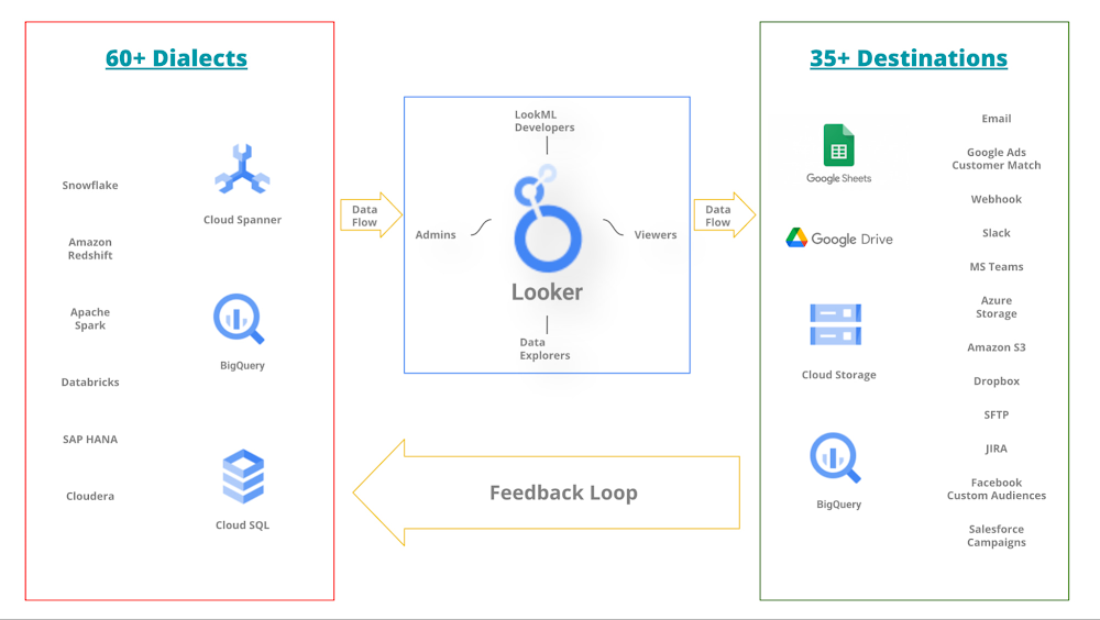
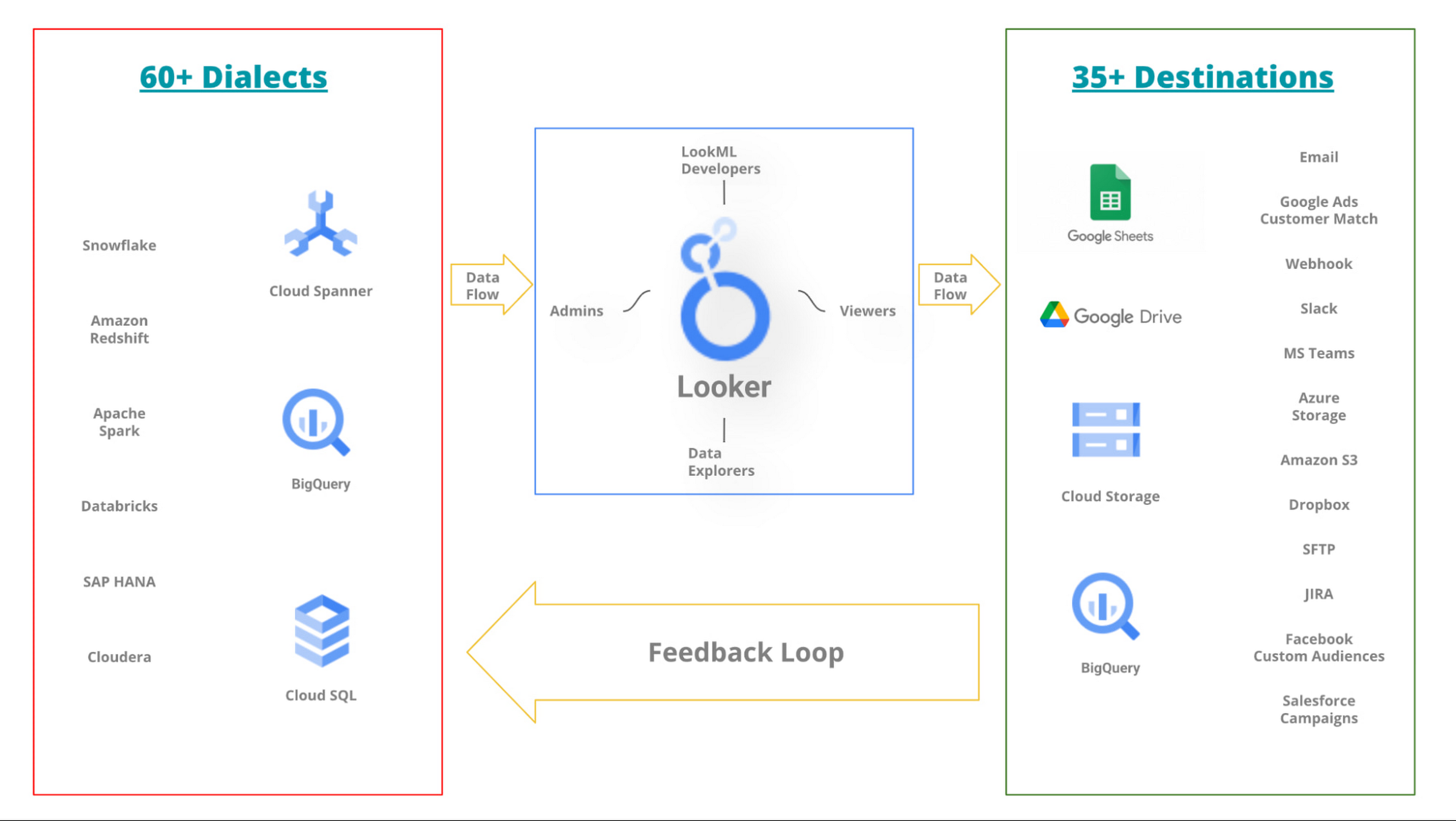
Nevertheless, a common goal across all these teams is keeping services running and downstream customers happy. In other words, the organization might be divided internally, however, they all have the mission to leverage the data to make better business decisions. Hence, despite silos and different subgoals, destiny for all these teams is intertwined for the organization to thrive. To support such a diverse set of data sources and the teams supporting them, Looker supports over 60 dialects (input from a data source) and over 35 destinations (output to a new data source).
Below is a simplified* picture of how the Looker ecosystem is central to a data-rich organization.
Simplified* Looker ecosystem in a data-rich environment
*The picture hides the complexity of team(s) accountable for each data source. It also hides how a data source may have dependencies on other sources. Looker Marketplace can also play an important role in your ecosystem.
What role can DevOps and SRE practices play?
In the most ideal state, all these teams will be in harmony as a single-threaded organization with all the internal processes so smooth that everyone is empowered to experiment (i.e. fail, learn, iterate and repeat all the time). With increasing organizational complexities, it is incredibly challenging to achieve such a state because there will be overhead and misaligned priorities. This is where we look up to the guiding principles of DevOps and SRE practices. In case you are not familiar with Google SRE practices, here is a starting point. The core of DevOps and SRE practices are mature communication and collaboration practices.
Let’s focus on the best practices which could help us with our Looker ecosystem.
Have joint goals. There should be some goals which are a shared responsibility across two or more teams. This helps establish a culture of psychological safety and transparency across teams.
Visualize how the data flows across the organization. This enables an understanding how each team plays their role and how to work with them better.
Agree on theGolden Signals (aka core metrics). These could mean data freshness, data accuracy, latency on centralized dashboards etc. These signals allow teams to set their error budgets and SLIs.
Agree on communication and collaboration methods that work across teams.
Focus on artifacts such as jointly owned documentations pages, shared roadmap items, reusable tooling, etc. For example, System Activity Dashboards could be made available to all the relevant stakeholders and supplemented with notes tailored to your organization.
Set up regular forums where commonly discussed agenda items include major changes, expected downtime and postmortems around the core metrics. Among other agenda items, you could define/refine a common set of standards, for example centrally defined labels, group_labels, descriptions, etc. in the LookML to ensure there is a single terminology across the board.
Promote informal sharing opportunities such as lessons learned, TGIFs, Brown bag sessions, and shadowing opportunities. Learning and teaching have an immense impact on how teams evolve. Teams often become closer with side projects that are slightly outside of their usual day-to-day duties.
Have mutually agreed upon change management practices. Each team has dependencies so making changes may have an impact on other teams. Why not plan those changes systematically? For example, getting common standards across the Advance deploy mode.
Promote continuous improvements. Keep looking for better, faster, cost-optimized versions of something important to the teams.
Revisit your data flow. After every major reorganization, ensure that organizational change has not broken the established mechanisms.
despite silos and different subgoals, destiny for all these teams is intertwined for the organization to thrive.
Are you over-engineering?
There is a possibility that in the process of maturing the ecosystem, we may end up in an overly engineered system – we may unintentionally add toil to the environment. These are examples of toil that often stem from communication gaps.
Meetings with no outcomes/action plans – This one is among the most common forms of toil, where the original intention of a meeting is no longer valid but the forum has not taken efforts to revisit their decision.
Unnecessary approvals – Being a single threaded team can often create unnecessary dependencies and your teams may lose the ability to make changes.
Unaligned maintenance windows – Changes across multiple teams may not be mutually exclusive hence if there is misalignment then it may create unforeseen impacts on the end user.
Fancy, but unnecessary tooling – Side projects, if not governed, may create unnecessary tooling which is not being used by the business. Collaborations are great when they solve real business problems, hence it is also required to refocus if the priorities are set right.
Gray areas – When you have a shared responsibility model, you also may end up in gray areas which are often gaps with no owner. This can lead to increased complexity in the long run. For example, having the flexibility to schedule content delivery still requires collaboration to reduce jobs with failures because it can impact the performance of your Looker instance.
Contradicting metrics – You may want to pay special attention to how teams are rewarded for internal metrics. For example, if a team focuses on accuracy of data and other one on freshness then at scale they may not align with one another.
Conclusion
To summarize, we learned how data is handled in large organizations with Looker at its heart unifying a universal semantic model. To handle large amounts of diverse data, teams need to start with aligned goals and commit to strong collaboration. We also learned how DevOps and SRE practices can guide us navigate through these complexities. Lastly, we looked at some side effects of excessively structured systems. To go forward from here, it is highly recommended to start with an analysis of how data flows under your scope and how mature the collaboration is across multiple teams.
In the past decade, we have experienced an unprecedented growth in the volume of data that can be captured, recorded and stored. In addition, the data comes in all shapes and forms, speeds and sources. This makes data accessibility, data accuracy, data compatibility, and data quality more complex than ever more. Which is why this year at our Data Engineer Spotlight, we wanted to bring together the Data Engineer Community to share important learning sessions and the newest innovations in Google Cloud.
Did you miss out on the live sessions? Not to worry – all the content is available on demand.
Interested in running a proof of concept using your own data? Sign up here forhands-on workshop opportunities.
#1: The next generation of Dataflow was announced, including Dataflow Go (allowing engineers to write core Beam pipelines in Go, data scientists to contribute with Python transforms, and data engineers to import standard Java I/O connectors). The best part, it all works together in a single pipeline. Dataflow ML (deploy easy ML models with PyTorch, TensorFlow, or stickit-learn to an application in real time), and Dataflow Prime (removes the complexities of sizing and tuning so you don’t have to worry about machine types, enabling developers to be more productive).
#2: Dataform Preview was announced (Q3 2022), which helps build and operationalize scalable SQL pipelines in BigQuery. My personal favorite part is that it follows software engineering best practices (version control, testing, and documentation) when managing SQL. Also, no other skills beyond SQL are required.
#3: Data Catalog is now part of Dataplex, centralizing security and unifying data governance across distributed data for intelligent data management, which can help governance at scale. Another great feature is that it has built-in AI-driven intelligence with data classification, quality, lineage, and lifecycle management.
#4: A how-to on BigQuery Migration Services was covered, which offers end-to-end migrations to BigQuery, simplifying the process of moving data into the cloud and providing tools to help with key decisions. Organizations are now able to break down their data silos. One great feature is the ability to accelerate migrations with intelligent automated SQL translations.
#5: The Google Cloud Hero Game was a gamified three hour Google Cloud training experience using hands-on labs to gain skills through interactive learning in a fun and educational environment. During the Data Engineer Spotlight, 50+ participants joined a live Google Meet call to play the Cloud Hero BigQuery Skills game, with the top 10 winners earning a copy of Visualizing Google Cloud by Priyanka Vergadia.
What was your biggest learning/takeaway from playing this Cloud Hero game?
It was brilliantly organized by the Cloud Analytics team at Google. The game day started off with the introduction and then from there we were introduced to the skills game. It takes a lot more than hands on to understand the concepts of BigQuery/SQL engine and I understood a lot more by doing labs multiple times. Top 10 winners receiving the Visualizing Google Cloud book was a bonus. – Shirish Kamath
Copy and pasting snippets of codes wins you competition. Just kidding. My biggest takeaway is that I get to explore capabilities of BigQuery that I may have not thought about before. – Ivan Yudhi
Would you recommend this game to your friends? If so, who would you recommend it to and why would you recommend it?
Definitely, there is so much need for learning and awareness of such events and games around the world, as the need for Data Analysis through the cloud is increasing. A lot of my friends want to upskill themselves and these kinds of games can bring a lot of new opportunities for them. – Karan Kukreja
What was your favorite part about the Cloud Hero BigQuery Skills game? How did winning the Cloud Hero BigQuery Skills game make you feel?
The favorite part was working on BigQuery Labs enthusiastically to reach the expected results and meet the goals. Each lab of the game has different tasks and learning, so each next lab was giving me confidence for the next challenge. To finish at the top of the leaderboard in this game makes me feel very fortunate. It was like one of the biggest milestones I have achieved in 2022. – Sneha Kukreja
Bitcoin has experienced tremendous price volatility in recent months. Traders are struggling to make sense of these patterns. Fortunately, new predictive analytics algorithms can make this easier.
The financial industry is becoming more dependent on machine learning technology with each passing day. Last summer, a report by Deloitte showed that more CFOs are using predictive analytics technology. Machine learning has helped reduce man-hours, increase accuracy and minimize human bias.
One of the biggest reasons people in the financial profession are investing in predictive analytics is to anticipate future prices of financial assets, such as stocks and bonds. The evidence demonstrating the effectiveness of predictive analytics for forecasting prices of these securities has been relatively mixed. However, the same principles can be applied to nontraditional assets more effectively, because they are in less efficient markets.
Many experts are using predictive analytics technology to forecast the future value of bitcoin. This is becoming a more popular idea as bitcoin becomes more volatile.
Can Predictive Analytics Really Help with Forecasting Bitcoin Price Movements Amidst Huge Market Volatility?
Bitcoin’s price is notoriously volatile. In the past, the value of a single Bitcoin has swung wildly by as much as $1,000 in a matter of days. As the market matures and more investors enter the space, we are beginning to see increased stability in prices. However, given the nature of cryptocurrency markets, it is still quite possible for prices to fluctuate rapidly. The good news is that predictive analytics technology can reduce risk exposure for these investors. For further information explore quantum code.
Predictive analytics algorithms are more effective at anticipating price patterns when they are designed with the right variables. There are a number of factors that can contribute to sudden changes in Bitcoin’s price that machine learning developers need to incorporate into their pricing models. These include:
News events: Positive or negative news about Bitcoin can have a significant impact on its price. For example, when China announced crackdowns on cryptocurrency exchanges in 2017, the price of Bitcoin fell sharply.Market sentiment: Investor sentiment can also drive price movements. When investors are bullish on Bitcoin, prices tend to rise. Conversely, when sentiment is bearish, prices tend to fall.Technical factors: Technical factors such as changes in trading volume, or the introduction of new trading platforms can also impact prices.
Predictive analytics technology helps traders assess these factors. , Chhaya Vankhede, a machine learning expert and author at Medium, developed a predictive analytics algorithm to predict bitcoin prices using LSTM. This algorithm proved to be surprisingly effective at forecasting bitcoin prices. However, they were not close to perfect, so she wants that more improvements need to be made.
Vankhede isn’t the only one that has developed predictive analytics models to predict bitcoin prices. Pratikkumar Prajapati of Cornell University published a study demonstrating the opportunity to forecast prices based on social media and news stories. This can be used to create more effective machine learning algorithms for traders.
Of course, it’s important to remember that Bitcoin is still a relatively new asset, and its price is subject to significant volatility. Therefore, predictive analytics is still an imperfect tool for projecting prices. In the long run, however, many believe that Bitcoin will become more stable as it continues to gain mainstream adoption.
Bitcoin’s price volatility has been a major source of concern for investors and observers alike. While the digital currency has seen its fair share of ups and downs, its overall trend has been positive, with prices steadily climbing since its inception. However, this doesn’t mean that there isn’t room for improvement.
There are a few key factors that contribute to Bitcoin’s volatility. Firstly, it is still a relatively new asset class, meaning that there are less data to work with when trying to predict future price movements. Secondly, the majority of Bitcoin users are speculators, rather than people using it as a currency to buy goods and services. This means that they are more likely to sell when prices rise, in order to cash in on their profits, leading to sharp price declines.
Finally, there is the question of trust. While the underlying technology of Bitcoin is sound, there have been a number of high-profile hacks and scams involving exchanges and wallets. This has led to some people losing faith in the digital currency, causing them to sell their holdings, leading to further price drops.
Despite these concerns, it is important to remember that Bitcoin is still in its early days. As more people adopt it and use it for everyday transactions, its price is likely to become more stable. In the meantime, investors should be prepared for periods of volatility. They can still minimize the risks by using predictive analytics strategically.
Positive Impacts of Bitcoin’s Price Volatility
Increased global awareness and media coverageMore people are interested in buying BitcoinThe price of Bitcoin becomes more stable over timeMore merchants start to accept Bitcoin as a payment methodGovernmental and financial institutions take notice of BitcoinThe value of Bitcoin increases
Negative Impacts of Bitcoin’s Price Volatility
People may lose interest in Bitcoin if the price is too volatileMerchants may be hesitant to accept Bitcoin if the price is volatileGovernmental and financial institutions may be reluctant to use Bitcoin if the price is unstableThe value of Bitcoin may decrease if the price is too volatileinvestors may be hesitant to invest in Bitcoin if the price is volatileSpeculators may take advantage of Bitcoin’s price volatility.
Bitcoin’s price is notoriously volatile, and this has caused many to wonder about the future of digital currency. Some have even called for it to be regulated in order to stabilize its value. However, others believe that Bitcoin’s volatility is actually a good thing, as it allows the market to correct itself and find true price discovery.
Bitcoin’s price is highly volatile compared to other asset classes. This means that its price can fluctuate rapidly in response to news and events. For example, the price of bitcoin fell sharply following the Mt. Gox hack in 2014 and the collapse of the Silk Road marketplace in 2013.
Investors must be aware of this risk when considering investing in bitcoin. While the potential for large gains is there, so is the potential for large losses. Bitcoin should only be a small part of an investment portfolio.
Predictive Analytics Technology is Necessary for Bitcoin Traders Trying to Minimize their Risk
Blockchain technology has changed our world in countless ways. Some of these changes have been beneficial, while others have been less helpful. For better or worse, we have to understand the impact it has had. One of the biggest changes the blockchain has created has been due to bitcoin mining.
Bitcoin Mining and the Blockchain Are Shaping Our World in Surprising Ways
Bitcoin mining is a process of verifying and adding transaction records to the public ledger called the blockchain. The blockchain is a distributed database that contains a record of all Bitcoin transactions that have ever been made. Every time a new transaction is made, it is added to the blockchain and verified by miners.
Miners are people or groups of people who use powerful computers to verify transactions and add them to the blockchain. Bitcoin miners are rewarded with newly created bitcoins and transaction fees for their work. Bitcode Prime provides more digital trading information.
Bitcoin mining has become increasingly popular over the years as the value of Bitcoin has surged. This wouldn’t have been possible without the blockchain. The blockchain plays a very important role in helping people buy bitcoin. As more people have started mining, the difficulty of finding new blocks has increased, making it more difficult for individual miners to earn rewards. However, large-scale miners have been able to find ways to keep their costs down and continue to profit from Bitcoin mining.
Bitcoin mining has had a large impact on the global economy. It has been estimated that the total energy consumption of Bitcoin mining could be as high as 7 gigawatts, which is equivalent to 0.21% of the world’s electricity consumption. This is because the blockchain is unfortunately not at all energy efficient. This estimate is based on a study that looked at the energy usage of different types of cryptocurrency mining.
The study found that Bitcoin mining is more energy-intensive than gold mining, and this difference is even larger when compared to other activities such as aluminum production or reserve banking. The large-scale nature of Bitcoin mining has led some experts to suggest that it could have a significant impact on the environment.
A recent report by the World Economic Forum estimated that the electricity used for Bitcoin mining could power all of the homes in the United Kingdom. This is based on the current rate of energy consumption and the number of homes in the country. The report also suggested that if the trend continues, Bitcoin mining could eventually use more electricity than is currently produced by renewable energy sources. The blockchain is unlikely to become more energy efficient without some major improvements. This can be a big problem as AI technology makes bitcoin even more popular in the UK.
The impact of Bitcoin mining on the environment has been a controversial topic. Some argue that it is a necessary evil that is needed to power the global economy, while others believe that it is a wasteful activity that should be banned. However, there is no denying that Bitcoin mining has had a significant impact on the world’s energy consumption and carbon footprint.
Bitcoin mining is a process that helps the Bitcoin network secure and validates transactions. It also creates new bitcoins in each block, similar to how a central bank prints new money. Miners are rewarded with bitcoin for their work verifying and committing transactions to the blockchain.
Bitcoin mining has become increasingly competitive as more people look to get involved in the cryptocurrency market. As a result, miners have had to invest more money in hardware and electricity costs in order to keep up with the competition.
This has led to some concerns about the environmental impact of Bitcoin mining, as the process requires a lot of energy. In particular, critics have pointed to the fact that most Bitcoin mining takes place in China, which relies heavily on coal-fired power plants.
However, it is worth noting that the vast majority of Bitcoin miners are using renewable energy sources. In fact, a recent study found that 78.79% of Bitcoin mining is powered by renewable energy.
This indicates that the environmental impact of Bitcoin mining is not as significant as some critics have claimed. Nevertheless, it is still important to keep an eye on the energy consumption of the Bitcoin network and ensure that steps are taken to improve efficiency where possible.
The 21st century has seen some incredible technological advances, and none more so than in the world of finance. The rise of digital currencies like Bitcoin has been nothing short of meteoric, and it doesn’t show any signs of slowing down. Bitcoin mining is the process by which new Bitcoins are created and transactions are verified on the blockchain. It’s a critical part of the Bitcoin ecosystem, but it comes with an environmental cost.
Bitcoin mining consumes a lot of energy. The exact amount is unknown, but it’s estimated that it could be as high as 7 gigawatts, which is about as much as the entire country of Bulgaria. This electricity consumption is contributing to climate change and damaging our planet.
Blockchain and Bitcoin Mining Have a Huge Impact on the Environment
There are a few ways to reduce the environmental impact of blockchain and Bitcoin mining. One is to use renewable energy sources, such as solar or wind power. Another is to use more efficient mining hardware. But the most important thing we can do is to raise awareness of the issue and work together to find a solution.
Pub/Sub’s ingestion of data into BigQuery can be critical to making your latest business data immediately available for analysis. Until today, you had to create intermediate Dataflow jobs before your data could be ingested into BigQuery with the proper schema. While Dataflow pipelines (including ones built with Dataflow Templates) get the job done well, sometimes they can be more than what is needed for use cases that simply require raw data with no transformation to be exported to BigQuery.
Starting today, you no longer have to write or run your own pipelines for data ingestion from Pub/Sub into BigQuery. We are introducing a new type of Pub/Sub subscription called a “BigQuery subscription” that writes directly from Cloud Pub/Sub to BigQuery. This new extract, load, and transform (ELT) path will be able to simplify your event-driven architecture. For Pub/Sub messages where advanced preload transformations or data processing before landing data in BigQuery (such as masking PII) is necessary, we still recommend going through Dataflow.
Get started by creating a new BigQuery subscription that is associated with a Pub/Sub topic. You will need to designate an existing BigQuery table for this subscription. Note that the table schema must adhere to certain compatibility requirements. By taking advantage of Pub/Sub topic schemas, you have the option of writing Pub/Sub messages to BigQuery tables with compatible schemas. If schema is not enabled for your topic, messages will be written to BigQuery as bytes or strings. After the creation of the BigQuery subscription, messages will now be directly ingested into BigQuery.
Better yet, you no longer need to pay for data ingestion into BigQuery when using this new direct method. You only pay for the Pub/Sub you use. Ingestion from Pub/Sub’s BigQuery subscription into BigQuery costs $50/TiB based on read (subscribe throughput) from the subscription. This is a simpler and cheaper billing experience compared to the alternative path via Dataflow pipeline where you would be paying for the Pub/Sub read, Dataflow job, and BigQuery data ingestion. See the pricing page for details.
To get started, you can read more about Pub/Sub’s BigQuery subscription or simply create a new BigQuery subscription for a topic using Cloud Console or the gcloud CLI.
R is one of the most widely used programming languages for statistical computing and machine learning. Many data scientists love it, especially for the rich world of packages from tidyverse, an opinionated collection of R packages for data science. Besides the tidyverse, there are over 18,000 open-source packages on CRAN, the package repository for R. RStudio, available as desktop version or on theGoogle Cloud Marketplace, is a popular Integrated Development Environment (IDE) used by data professionals for visualization and machine learning model development.
Once a model has been built successfully, a recurring question among data scientists is: “How do I deploy models written in the R language to production in a scalable, reliable and low-maintenance way?”
In this blog post, you will walk through how to use Google Vertex AI to train and deploy enterprise-grade machine learning models built with R.
Overview
Managing machine learning models on Vertex AI can be done in a variety of ways, including using the User Interface of the Google Cloud Console, API calls, or the Vertex AI SDK for Python.
Since many R users prefer to interact with Vertex AI from RStudio programmatically, you will interact with Vertex AI through the Vertex AI SDK via the reticulate package.
Train a model locally and import it as a custom model into Vertex AI Model Registry, from where it can be deployed to an endpoint for serving predictions.
Create a TrainingPipeline that runs a CustomJob and imports the resulting artifacts as a Model.
In this blog post, you will use the second method and train a model directly in Vertex AI since this allows us to automate the model creation process at a later stage while also supporting distributed hyperparameter optimization.
The process of creating and managing R models in Vertex AI comprises the following steps:
Enable Google Cloud Platform (GCP) APIs and set up the local environment
Create custom R scripts for training and serving
Create a Docker container that supports training and serving R models with Cloud Build and Container Registry
Train a model using Vertex AI Training and upload the artifact to Google Cloud Storage
Create a model endpoint on Vertex AI Prediction Endpoint and deploy the model to serve online prediction requests
To showcase this process, you train a simple Random Forest model to predict housing prices on the California housing data set. The data contains information from the 1990 California census. The data set is publicly available from Google Cloud Storage at gs://cloud-samples-data/ai-platform-unified/datasets/tabular/california-housing-tabular-regression.csv
The Random Forest regressor model will predict a median housing price, given a longitude and latitude along with data from the corresponding census block group. A block group is the smallest geographical unit for which the U.S. Census Bureau publishes sample data (a block group typically has a population of 600 to 3,000 people).
Environment Setup
This blog post assumes that you are either using Vertex AI Workbench with an R kernel or RStudio. Your environment should include the following requirements:
The Google Cloud SDK
Git
R
Python 3
Virtualenv
To execute shell commands, define a helper function:
Next, you define variables to support the training and deployment process, namely:
PROJECT_ID: Your Google Cloud Platform Project ID
REGION: Currently, the regions us-central1, europe-west4, and asia-east1 are supported for Vertex AI; it is recommended that you choose the region closest to you
BUCKET_URI: The staging bucket where all the data associated with your dataset and model resources are stored
DOCKER_REPO: The Docker repository name to store container artifacts
IMAGE_NAME: The name of the container image
IMAGE_TAG: The image tag that Vertex AI will use
IMAGE_URI: The complete URI of the container image
When you initialize the Vertex AI SDK for Python, you specify a Cloud Storage staging bucket. The staging bucket is where all the data associated with your dataset and model resources are retained across sessions.
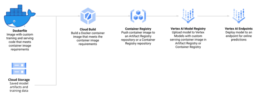
Create Docker container image for training and serving R models
The docker file for your custom container is built on top of the Deep Learning container — the same container that is also used for Vertex AI Workbench. In addition, you add two R scripts for model training and serving, respectively.
Before creating such a container, you enable Artifact Registry and configure Docker to authenticate requests to it in your region.
code_block[StructValue([(u’code’, u’# filename: Dockerfile – container specifications for using R in Vertex AIrnFROM gcr.io/deeplearning-platform-release/r-cpu.4-1:latestrnrnWORKDIR /rootrnrnCOPY train.R /root/train.RrnCOPY serve.R /root/serve.Rrnrn# Install FortranrnRUN apt-get updaternRUN apt-get install gfortran -yyrnrn# Install R packagesrnRUN Rscript -e “install.packages(‘plumber’)”rnRUN Rscript -e “install.packages(‘randomForest’)”rnrnEXPOSE 8080′), (u’language’, u”), (u’caption’, <wagtail.wagtailcore.rich_text.RichText object at 0x3ead93a41450>)])]
Next, create the file train.R, which is used to train your R model. The script trains a randomForest model on the California Housing dataset. Vertex AI sets environment variables that you can utilize, and since this script uses a Vertex AI managed dataset, data splits are performed by Vertex AI and the script receives environment variables pointing to the training, test, and validation sets. The trained model artifacts are then stored in your Cloud Storage bucket.
code_block[StructValue([(u’code’, u’#!/usr/bin/env Rscriptrn# filename: train.R – train a Random Forest model on Vertex AI Managed Datasetrnlibrary(tidyverse)rnlibrary(data.table)rnlibrary(randomForest)rnSys.getenv()rnrn# The GCP Project IDrnproject_id <- Sys.getenv(“CLOUD_ML_PROJECT_ID”)rnrn# The GCP Regionrnlocation <- Sys.getenv(“CLOUD_ML_REGION”)rnrn# The Cloud Storage URI to upload the trained model artifact tornmodel_dir <- Sys.getenv(“AIP_MODEL_DIR”)rnrn# Next, you create directories to download our training, validation, and test set into.rndir.create(“training”)rndir.create(“validation”)rndir.create(“test”)rnrn# You download the Vertex AI managed data sets into the container environment locally.rnsystem2(“gsutil”, c(“cp”, Sys.getenv(“AIP_TRAINING_DATA_URI”), “training/”))rnsystem2(“gsutil”, c(“cp”, Sys.getenv(“AIP_VALIDATION_DATA_URI”), “validation/”))rnsystem2(“gsutil”, c(“cp”, Sys.getenv(“AIP_TEST_DATA_URI”), “test/”))rnrn# For each data set, you may receive one or more CSV files that you will read into data frames.rntraining_df <- list.files(“training”, full.names = TRUE) %>% map_df(~fread(.))rnvalidation_df <- list.files(“validation”, full.names = TRUE) %>% map_df(~fread(.))rntest_df <- list.files(“test”, full.names = TRUE) %>% map_df(~fread(.))rnrnprint(“Starting Model Training”)rnrf <- randomForest(median_house_value ~ ., data=training_df, ntree=100)rnrfrnrnsaveRDS(rf, “rf.rds”)rnsystem2(“gsutil”, c(“cp”, “rf.rds”, model_dir))’), (u’language’, u”), (u’caption’, <wagtail.wagtailcore.rich_text.RichText object at 0x3ead920dc110>)])]
Next, create the file serve.R, which is used for serving your R model. The script downloads the model artifact from Cloud Storage, loads the model artifacts, and listens for prediction requests on port 8080. You have several environment variables for the prediction service at your disposal, including:
AIP_HEALTH_ROUTE: HTTP path on the container that AI Platform Prediction sends health checks to.
Next, you build the Docker container image on Cloud Build — the serverless CI/CD platform. Building the Docker container image may take 10 to 15 minutes.
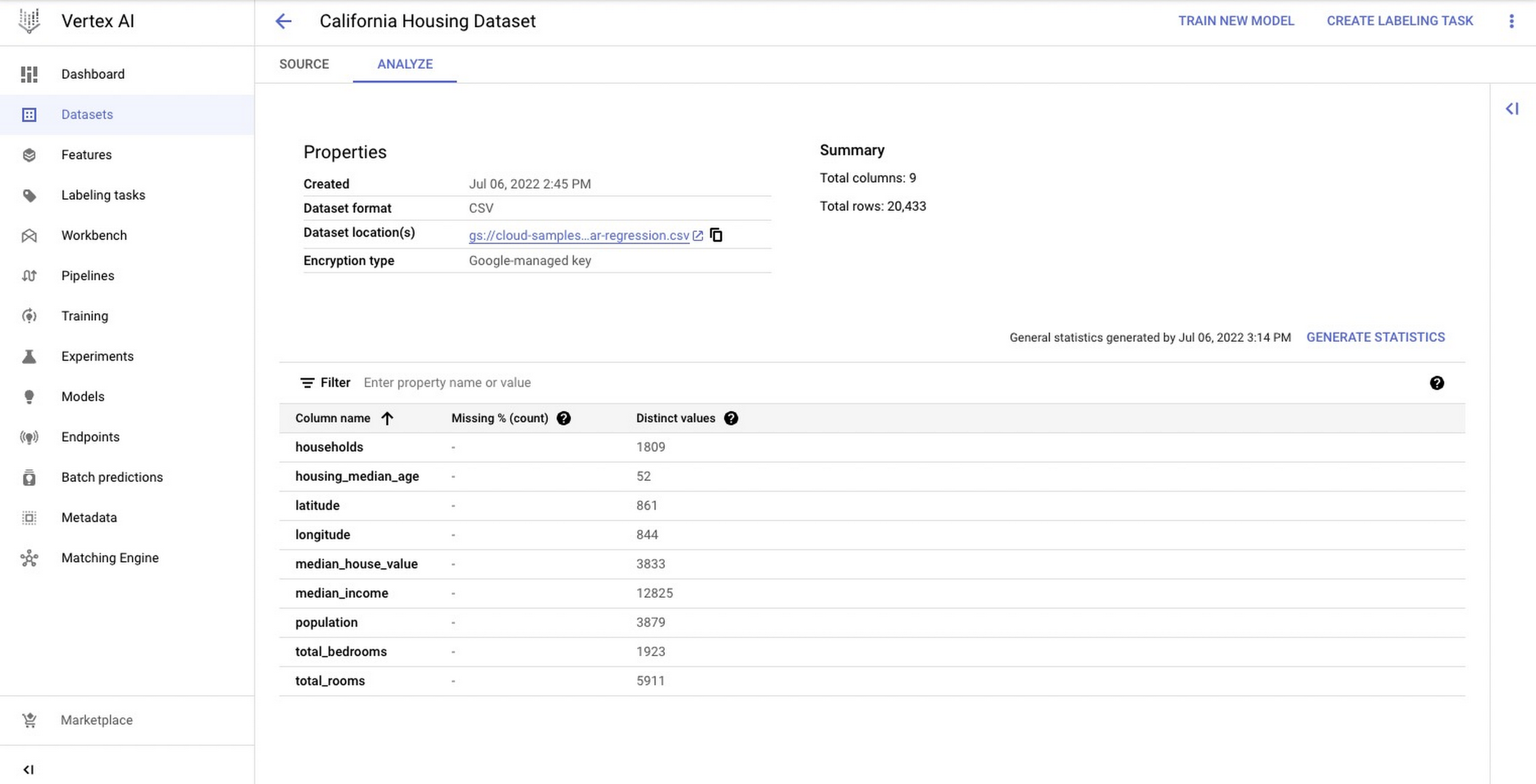
You create a Vertex AI Managed Dataset to have Vertex AI take care of the data set split. This is optional, and alternatively you may want to pass the URI to the data set via environment variables.
The next screenshot shows the newly created Vertex AI Managed dataset in Cloud Console.
Train R Model on Vertex AI
The custom training job wraps the training process by creating an instance of your container image and executing train.R for model training and serve.R for model serving.
Note: You use the same custom container for both training and serving.
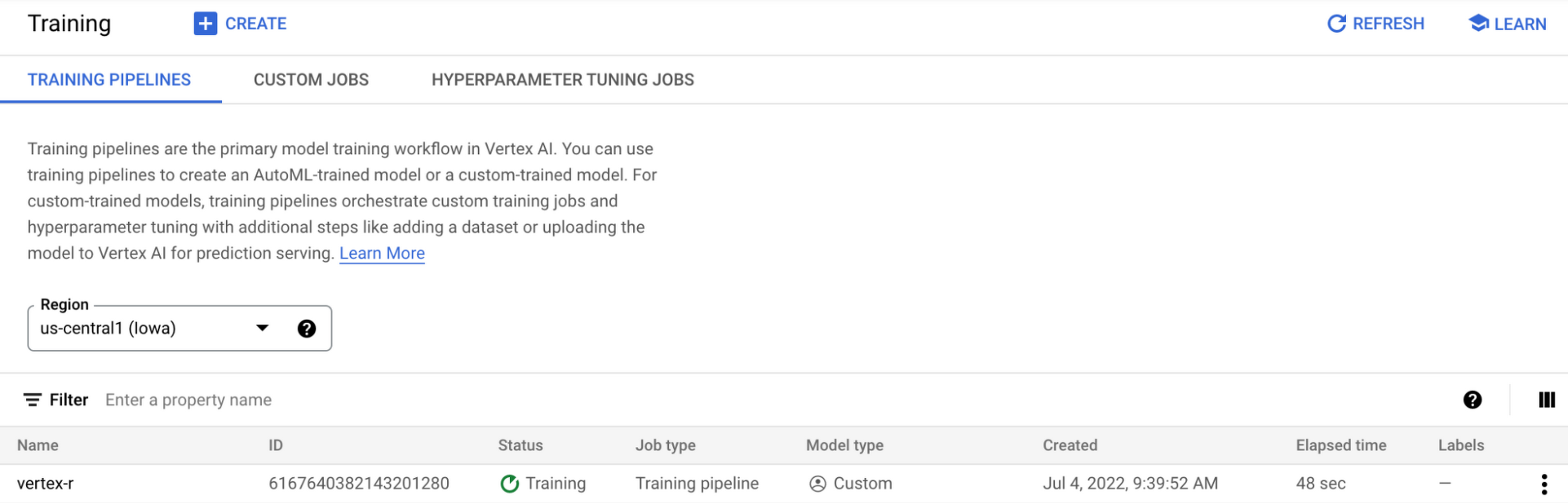
To train the model, you call the method run(), with a machine type that is sufficient in resources to train a machine learning model on your dataset. For this tutorial, you use a n1-standard-4 VM instance.
The model is now being trained, and you can watch the progress in the Vertex AI Console.
Provision an Endpoint resource and deploy a Model
You create an Endpoint resource using the Endpoint.create() method. At a minimum, you specify the display name for the endpoint. Optionally, you can specify the project and location (region); otherwise the settings are inherited by the values you set when you initialized the Vertex AI SDK with the init() method.
In this example, the following parameters are specified:
display_name: A human readable name for the Endpoint resource.
project: Your project ID.
location: Your region.
labels: (optional) User defined metadata for the Endpoint in the form of key/value pairs.
You can deploy one of more Vertex AI Model resource instances to the same endpoint. Each Vertex AI Model resource that is deployed will have its own deployment container for the serving binary.
Next, you deploy the Vertex AI Model resource to a Vertex AI Endpoint resource. The Vertex AI Model resource already has defined for it the deployment container image. To deploy, you specify the following additional configuration settings:
The machine type.
The (if any) type and number of GPUs.
Static, manual or auto-scaling of VM instances.
In this example, you deploy the model with the minimal amount of specified parameters, as follows:
model: The Model resource.
deployed_model_displayed_name: The human readable name for the deployed model instance.
machine_type: The machine type for each VM instance.
Due to the requirements to provision the resource, this may take up to a few minutes.
Note: For this example, you specified the R deployment container in the previous step of uploading the model artifacts to a Vertex AI Model resource.
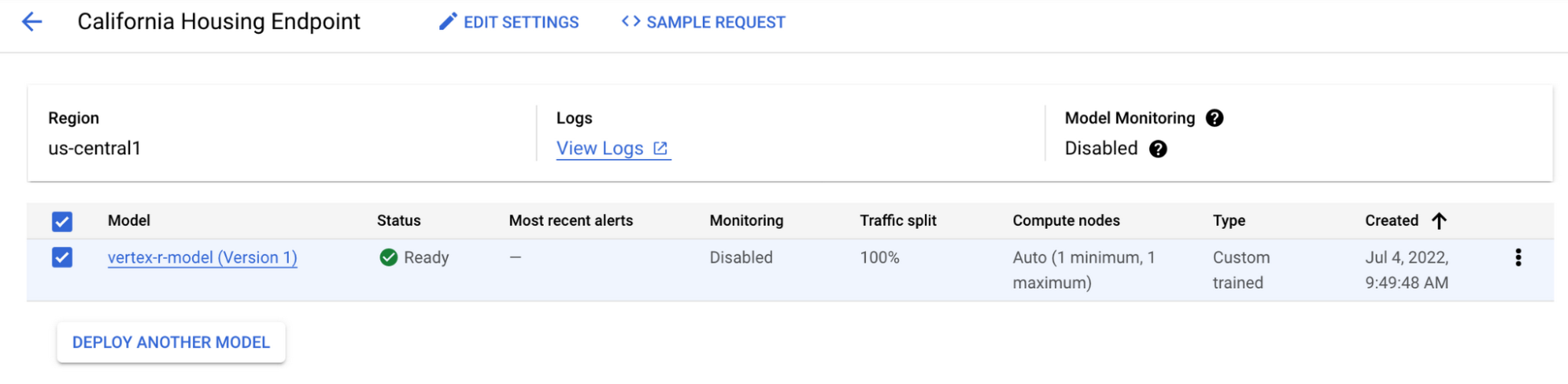
The model is now being deployed to the endpoint, and you can see the result in the Vertex AI Console.
Make predictions using newly created Endpoint
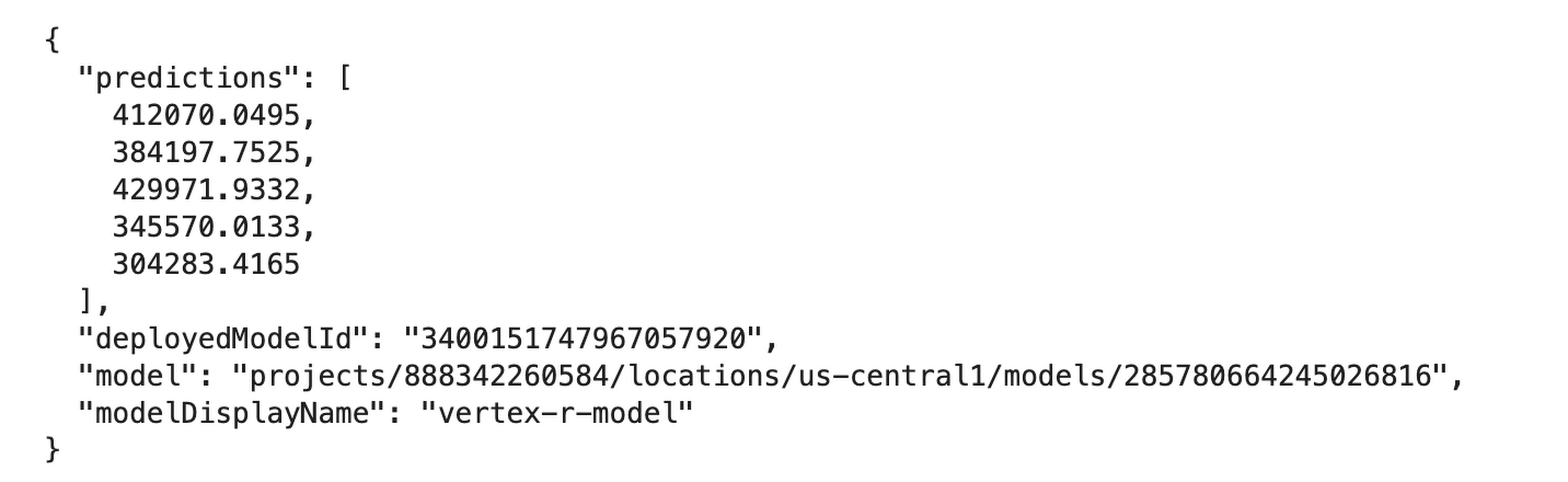
Finally, you create some example data to test making a prediction request to your deployed model. You use five JSON-encoded example data points (without the label median_house_value) from the original data file in data_uri. Finally, you make a prediction request with your example data. In this example, you use the REST API (e.g., Curl) to make the prediction request.
The endpoint now returns five predictions in the same order the examples were sent.
Cleanup
To clean up all Google Cloud resources used in this project, you can delete the Google Cloud project you used for the tutorial or delete the created resources.
code_block[StructValue([(u’code’, u’endpoint$undeploy_all()rnendpoint$delete()rndataset$delete()rnmodel$delete()rnjob$delete()’), (u’language’, u”), (u’caption’, <wagtail.wagtailcore.rich_text.RichText object at 0x3ead93078150>)])]
Summary
In this blog post, you have gone through the necessary steps to train and deploy an R model to Vertex AI. For easier reproducibility, you can refer to this Notebook on GitHub
Acknowledgements
This blog post received contributions from various people. In particular, we would like to thank Rajesh Thallam for strategic and technical oversight, Andrew Ferlitsch for technical guidance, explanations, and code reviews, and Yuriy Babenko for reviews.


