In retail, the distinction between physical and digital has blurred, and the home improvement sector is no exception. At Kingfisher, our retail banners include B&Q, Castorama, Brico Dépôt, and Screwfix, and our customers expect a seamless shopping experience whether they shop with us online or in store.
From product recommendations to delivery suggestions to location-based services, the technology required to meet these changing expectations is all powered by data. And to effectively deliver for our customers, that data needs to be highly available, highly accurate, and highly optimized. It needs to be gold standard.
In November 2022, we signed a five-year strategic partnership with Google Cloud to accelerate the migration of our huge on-premises SAP workloads to the cloud. By moving away from a tightly coupled, monolithic architecture, our goal was to improve our resilience and strengthen our data platform to unleash the full potential of our data, giving us the resilience and agility we need to power our growth.
The right platform — and people — to help us do it ourselves
Data speed and quality are critical to helping us achieve our goals, with data platforms, recommendation engines, sophisticated machine learning, and the ability to quickly ingest and curate content, all key to our future plans. Partnering with Google Cloud helps us to unlock this potential, with Google Cloud Marketplace also offering a critical capability to help us simplify procurement.
One of the most important factors in our decision to partner with Google Cloud was the expertise. Google Cloud not only brings a specific set of functionality and services that are well suited to our needs, but a team of people behind those solutions who understand our industry. They know our needs and goals, and can help us work through our challenges. And as we continue to migrate our workloads and build our architecture, the Google Cloud team is fully engaged, working closely with us in a meeting of minds.
Unleashing data’s potential to meet customer expectations
This partnership has already started to deliver results. By abstracting the data away from our core platform, we are now able to use it more productively for our business needs, and we’re currently working on some use cases around supply chain visibility. One such project enables us to dynamically price products according to various live promotions, so that we can react to the market with more agility.
This is only possible because we’ve been able to separate the data from our SAP system and run it through Google Cloud solutions such as BigQuery and Cloud Storage, enabling us to provide a more personalized shopping experience. Plans are now underway to use our product and sales data to create a new, real-time order system to greatly improve stock accuracy, as well as scaling up B&Q’s online marketplace from 700,000 products to 4 million (Kingfisher’s H1 2023/23 Financial Results).
Facing the future with a solid foundation
The future of digital retail is highly compute-intensive, requiring a level of real-time data processing near equivalent to that needed to power a major stock market. Working with Google Cloud gives us the processing power to use our data to its full potential, freeing us to focus on what we do best: offering the best home improvement proposition to our customers.
The growing suite of AI solutions in Google Cloud adds another dimension to our ability to leverage data, which will be increasingly important to enhancing the customer experience. Vertex AI, for example, is already allowing us to optimize our product pages, so that customers can visualize products in different scenarios and make a more informed purchasing decision. Throughout the business, AI is improving and speeding up our internal processes, which ultimately allows us to better serve our customers.
It’s no secret the retail industry is evolving at pace. With Google Cloud, we now have the agility, the support, and the data platform to create more seamless customer experiences both in stores and online.
In the UK there is a requirement for certain utility businesses to maintain a Priority Services Register (PSR) — a free support service to provide extra help to customers who need it or have particular personal circumstances which mean they may be harmed in case of an interruption to their utilities service.
We started looking into PSRs and other safeguarding initiatives. Information is often siloed in different organisations, which makes it difficult to access the data needed to provide critical support. Recent research indicates fewer than 20% of UK adults are aware of the PSR, which can mean records are incomplete, limiting both the delivery of the service and how well it is delivered.
A potential approach to serving the more vulnerable while addressing security and data privacy challenges uses a publish subscribe model (illustrated in the diagram below). People who own information (publishers) put it into the exchange for other people (subscribers) to access. In many cases organizations will be both. Organizations contribute their part of the jigsaw puzzle to help build a more comprehensive picture for all. Participants retain control of the information they publish.
Data is published on an exchange, which authorized subscribers can access, with privacy and security controls built in. Subscribers can then overlay their own data and perform analytics.
The private exchange model makes it possible to restrict access to the system, which in turn allows participants to share controlled elements of a PSR. We are doing this in trials underway with a few organizations, including the Citizens Advice Greater Manchester.
Using an exchange hub, different organizations can publish their PSR information. Data that was previously only accessible by each then becomes available to everyone on the exchange to use for the benefit of all. This can give subscribers a bigger and more comprehensive view, with controls being constantly applied to help ensure that Personal Identifiable Information is being managed appropriately.
Putting this into practice means, for example, you can display your PSR on a map. You can then gather and add additional information from electricity, gas, water utilities, emergency services, local authorities, and charities. The image below provides an example of PSR data being combined with Office for National Statistics data on average income to help better identify areas of potential fuel poverty.
It is then possible to go a step further by applying predictive analytics techniques. For example, what if inflation were to increase to 10%? The system would show you what that could look like and places where fuel poverty is likely to increase. There are many data sets available which can deliver incredible value when applied in this way. Another example might be to identify those in an area living in poorly insulated homes or on floodplains.
The technology offers a wealth of unexplored opportunities to make life better for people who need extra support.
Contact us to discover how you can embark on a journey towards a safer, and more inclusive future.
YugabyteDB, a distributed SQL database, when combined with BigQuery, tackles data fragmentation, data integration, and scalability issues businesses face.
It ensures that data is well-organized and not scattered across different places, making it easier to use in BigQuery for analytics. YugabyteDB’s ability to grow with the amount of data helps companies handle more information without slowing down. It also maintains consistency in data access, crucial for reliable results in BigQuery’s complex queries. The streamlined integration enhances overall efficiency by managing and analyzing data from a single source, reducing complexity. This combination empowers organizations to make better decisions based on up-to-date and accurate information, contributing to their success in the data-driven landscape.
BigQuery is renowned for its ability to store, process, and analyze vast datasets using SQL-like queries. As a fully managed service with seamless integration into other Google Cloud Platform services, BigQuery lets users scale their data operations to petabytes. It also provides advanced analytics, real-time dashboards, and machine learning capabilities. By incorporating YugabyteDB into the mix, users can further enhance their analytical capabilities and streamline their data pipeline.
YugabyteDB is designed to deliver scale, availability and enterprise-grade RDBMS capabilities for mission-critical transactional applications. It is a powerful cloud-native database that thrives in any cloud environment. With its support for multi-cloud and hybrid cloud deployment, YugabyteDB seamlessly integrates with BigQuery using the YugabyteDB CDC Connector and Apache Kafka. This integration enables the real-time consumption of data for analysis without the need for additional processing or batch programs.
Benefits of BigQuery integration with YugabyteDB
Integrating YugabyteDB with BigQuery offers numerous benefits. Here are the top six.
Real-time data integration: YugabyteDB’s Change Data Capture (CDC) feature synchronizes data changes in real-time between YugabyteDB and BigQuery tables. This seamless flow of data enables real-time analytics, ensuring that users have access to the most up-to-date information for timely insights.Data accuracy: YugabyteDB’s CDC connector ensures accurate and up-to-date data in BigQuery. By capturing and replicating data changes in real-time, the integration guarantees that decision-makers have reliable information at their disposal, enabling confident and informed choices.Scalability: Both YugabyteDB and BigQuery are horizontally scalable solutions capable of handling the growing demands of businesses. As data volumes increase, these platforms can seamlessly accommodate bigger workloads, ensuring efficient data processing and analysis.Predictive analytics: By combining YugabyteDB’s transactional data with the analytical capabilities of BigQuery, businesses can unlock the potential of predictive analytics. Applications can forecast trends, predict future performance, and proactively address issues before they occur, gaining a competitive edge in the market.Multi-cloud and hybrid cloud deployment: YugabyteDB’s support for multi-cloud and hybrid cloud deployments adds flexibility to the data ecosystem. This allows businesses to retrieve data from various environments and combine it with BigQuery, creating a unified and comprehensive view of their data.
By harnessing the benefits of YugabyteDB and BigQuery integration, businesses can supercharge their analytical capabilities, streamline their data pipelines, and gain actionable insights from their large datasets. Whether you’re looking to make data-driven decisions, perform real-time analytics, or leverage predictive analytics, combining YugabyteDB and BigQuery is a winning combination for your data operations.
Key use cases for YugabyteDB and BigQuery integration
YugabyteDB’s Change Data Capture (CDC) with BigQuery serves multiple essential use cases. Let’s focus on two key examples.
1.Industrial IoT (IIoT): In IIoT, streaming analytics is the continuous analysis of data records as they are generated. Unlike traditional batch processing, which involves collecting and analyzing data at regular intervals, streaming analytics enables real-time analysis of data from sources like sensors/actuators, IoT devices and IoT gateways. This data can then be written into YugabyteDB with high throughput and then streamed continuously to BigQuery Tables for advanced analytics using Google Vertex AI or other AI programs.
Examples of IIoT Stream Analytics
BigQuery can process and analyze data from industrial IoT devices, enabling efficient operations and maintenance. Two real-world examples include:
Supply chain optimization: Analyze data from IoT-enabled tracking devices to monitor inventory, track shipments, and optimize logistics operations.Energy efficiency: Analyze data from IoT sensors and meters to identify energy consumption patterns to optimize usage and reduce costs.
2. Equipment predictive maintenance analytics: In various industries such as manufacturing, telecom, and instrumentation, equipment predictive maintenance analytics is a common and important use case. YugabyteDB plays a crucial role in collecting and storing equipment notifications and performance data in real time. This enables the seamless generation of operational reports for on-site operators, providing them with current work orders and notifications.
Maintenance analytics is important for determining equipment lifespan and identifying maintenance requirements. YugabyteDB CDC facilitates the integration of analytics data residing in BigQuery. By pushing the stream of notifications and work orders to BigQuery tables, historical data accumulates, enabling the development of machine learning or AI models. These models can be fed back to YugabyteDB for tracking purposes, including failure probabilities, risk ratings, equipment health scores, and forecasted inventory levels for parts. This integration not only enables advanced analytics but also helps the OLTP database (in this case, YugabyteDB) store the right data for the site engineers or maintenance personnel in the field.
So now let’s walk through how easy it is to integrate YugabyteDB with BigQuery using CDC.
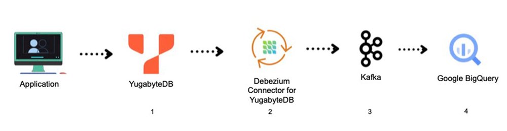
Integration architecture of YugabyteDB to BigQuery
The diagram below (Figure 1) shows the end-to-end integration architecture of YugabyteDB to BigQuery.
Figure 1 – End to End Architecture
The table below shows the data flow sequences with their operations and tasks performed.
Install and set up YugabyteDB CDC and Debezium connector
Ensure YugabyteDB CDC is configured to capture changes in the database and is running (as per the above architecture diagram) along with its dependent components. You should see a Kafka topic name and group name as per this document; it will appear in the streaming logs either through CLI or via Kafka UI (e.g. if you used KOwl).
Download and configure BigQuery Connector
Download the BigQuery Connector . Unzip and add the JAR files to YugabyteDB’s CDC (Debezium Connector) Libs folder (e.g. /kafka/libs). Then restart the Docker container
Set up BigQuery in Google Cloud
Setting up BigQuery in Google Cloud benefits both developers and DBAs by providing a scalable, serverless, and integrated analytics platform. It simplifies data analytics processes, enhances collaboration, ensures security and compliance, and supports real-time processing, ultimately contributing to more effective and efficient data-driven decision-making.
Follow these five steps to set up BigQuery in Google Cloud.
Create a Google Cloud Platform account. If you don’t already have one, create a Google Cloud Platform account by visiting the Google Cloud Console and following the prompts.Create a new project (if you don’t already have one). Once you’re logged into the Google Cloud Console, create a new project by clicking the “Select a Project” dropdown menu at the top of the page and clicking on “New Project”. Follow the prompts to set up your new project.Enable billing (if you haven’t done it already). NOTE: Before you can use BigQuery, you need to enable billing for your Google Cloud account. To do this, navigate to the “Billing” section of the Google Cloud Console and follow the prompts.Enable the BigQuery API: To use BigQuery, you need to enable the BigQuery API for your project. To do this, navigate to the “APIs & Services” section of the Google Cloud Console and click on “Enable APIs and Services”. Search for “BigQuery” and click the “Enable” button..Create a Service Account and assign BigQuery roles in IAM (Identity and Access Management): As shown in Figure 4, create a service account and assign the IAM role for Big Query. The following roles are mandatory to create a BigQuery table:BigQuery Data EditorBigQuery Data Owner
Figure 2 – Google Cloud – Service Account for BigQuery
After creating a service account, you will see the details (as shown in Figure 3). Create a private and public key for the service account and download it in your local machine. It needs to be copied to YugabyteDB’s CDC Debezium Docker container in a designated folder (e.g., “/kafka/balabigquerytesting-cc6cbd51077d.json”). This is what you refer to while deploying the connector.
Figure 3 – Google Cloud – Generate Key for the Service Account
2. Deploy the configuration for the BigQuery connector
Source Connector
Create and deploy the source connector (as shown below), change the database hostname, database master addresses, database user, password, database name, logical server name and table include list and StreamID according to your CDC configuration (refer code block highlighted in yellow).
The configuration below shows a sample BigQuerySink connector. The topic name, Google project, dataset name, default dataset name — highlighted in yellow — need to be replaced according to your specific configuration.
The key file fields contain the private key location of your Google project, and it needs to be kept in the YugabyteDB’s CDC Debezium Docker connector folder. (e.g. /kafka)
After deployment, the table name (e.g. dbserver11_public_testcdc) will be created in BigQuery automatically (see below).
Figure 4 – Data stored in the BigQuery Table
Figure 5 – BigQuery – Execution Details for a sample BigQuery table is shown below.
Figure 6 – Query Execution Details
Conclusion and summary
Following the steps above is all it takes to integrate YugabyteDB’s CDC connector with BigQuery.
Combining YugabyteDB OLTP data with BigQuery data can benefit an application in a number of ways (e.g. real-time analytics, advanced analytics with machine learning, historical analysis and data warehousing and reporting). YugabyteDB holds the transactional data that is generated by an application in real-time, while BigQuery data is typically large, historical data sets that are most often used for analysis. By combining these two types of data, an application can leverage the strengths of both to provide real-time insights and support better, quicker, more accurate and informed decision-making.
Editor’s note: The post is part of a series showcasing our partners, and their solutions, that are Built with BigQuery.
Data collaboration, the act of gathering and connecting data from various sources to unlock combined data insights, is the key to reaching, understanding, and expanding your audience. And enabling global businesses to accurately connect, unify, control, and activate data across different channels and devices will ultimately optimize customer experiences and drive better results.
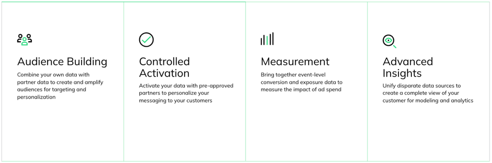
LiveRamp is a leader in data collaboration, with clients that span every major industry. One of LiveRamp’s enterprise platforms, Safe Haven, helps enterprises do more with their data, and is especially valuable for brands constructing clean room environments for their partners and retail media networks. It enables four universal use cases to facilitate better customer experiences:
The core challenge: Creating accurate cross-channel marketing analytics
As brand marketers accelerate their move to the cloud, they struggle to execute media campaigns guided by data and insights. This is due to challenges in building effective cross-channel marketing analytics, which need to overcome the following hurdles:
Lack of a common key to accurately consolidate and connect data elements and behavioral reports from different data sources that should be tied to the same consumer identity. Such a “join key” can not be a constructed internal record ID, as it must be semantically rich enough to work for both individual and household-level data across all the brand’s own prospects and customers, and across all of the brand’s partner data (e.g., data from publishers, data providers, co-marketing partners, supply-chain providers, agency teams).Reduced data availability from rising consumer authentication requirements makes it difficult to reach a sufficient sample volume for accurately driving recommendation and personalization engines, creating lookalikes, or for creating unbiased data inputs for incorporating into machine learning training.Brand restrictions on analytic operations to guard against data leaks of sensitive consumer personally-identifiable information (PII). By reducing operational access to consumer data, brands increase their data protections but decrease their data science team’s ability to discover key insights and perform cross-partner audience measurements.Decreased partner collaboration from using weak individual record identifiers, such as hashed emails, as the basis for record matching. Hashed emails are often produced by default by many customer data platforms (CDPs), but these identifiers are insecure due to their easy-reversibility and have limited capacity to connect the same individual and household across partners.
LiveRamp solves these challenges for marketers by building a suite of dedicated data connectivity tools and services centered on Google’s BigQuery ecosystem — with the objective of creating the ultimate open data-science environment for marketing analytics on Google Cloud.
The resulting LiveRamp Safe Haven environment is deployed, configured and customized for each client’s Google Cloud instance. The solution is scalable, secure and future-proof by being deployed alongside Google’s BigQuery ecosystem. As Google Cloud technology innovation continues, users of Safe Haven are able to naturally adopt new analytic tools and libraries enabled by BigQuery.
All personally-identifiable data in the environment is automatically processed and replaced with LiveRamp’s brand-encoded pseudonymized identifiers, known as RampIDs:
These identifiers are derived from LiveRamp’s decades of dedicated work on consumer knowledge and device-identity knowledge graphs. LiveRamp’s identifiers represent secure people-based individual and household-level IDs that let data scientists connect audience records, transaction records, and media behavior records across publishers and platforms.Because these RampIDs are based on actual demographic knowledge, these identifiers can connect data sets with real person-centered accuracy and higher connectivity than solutions that rely on string matching alone.RampIDs are supported in Google Ads, Google’s Ads Data Hub, and hundreds of additional leading destinations including TV and Connected TV, Walled Gardens, ecommerce platforms, and all leading social and programmatic channels.
The Safe Haven data, because of its pseudonymization, presents a much safer profile for analysts working in the environment, with little risk to insider threats due to PII removal, a lockdown of data exports, transparent activity logging, and Google Cloud’s powerful encryption and role-based permissioning.
LiveRamp’s Safe Haven solutions on Google Cloud have been deployed by many leading brands globally, especially brands in retail, CPG, pharma, travel, and entertainment. Success for all of these brands is due in large part to the combination of the secure BigQuery environment and the ability to increase data connectivity with LiveRamp’s RampID ecosystem partners.
One powerful example in the CPG space is the success achieved by a large CPG client who needed to enrich their understanding of consumer product preferences, and piloted a focused effort to assess the impact of digital advertising on audience segments and their path to purchase at one large retailer.
Using Safe Haven running on BigQuery, they were able to develop powerful person-level insights, create new optimized audience segments based on actual in-store product affinities, and greatly increase their direct addressability to over a third of their regional purchasers. The net result was a remarkable 24.7% incremental lift over their previous campaigns running on Google and on Facebook.
Built with BigQuery: How Safe Haven empowers analysts and marketers
Whether you’re a marketer activating media audience segments, or a data scientist using analytics across the pseudonymized and connected data sets, LiveRamp Safe Haven delivers the power of BigQuery to either end of the marketing function.
Delivering BigQuery to data scientists and analysts
Creating and configuring an ideal environment for marketing analysts is a matter of selecting and integrating from the wealth of powerful Google and partner applications, and uniting them with common data pipelines, data schemas, and processing pipelines. An example configuration LiveRamp has used for retail analysts combines Jupyter, Tableau, Dataproc and BigQuery as shown below:
Data scientists and analysts need to work iteratively and interactively to analyze and model the LiveRamp-connected data. To do this, they have the option of using either the SQL interface through the standard BigQuery console, or for more complex tasks, they can write Python spark jobs inside a custom JupyterLab environment hosted on the same VM that utilizes a Dataproc cluster for scale.
They also need to be able to automate, schedule and monitor jobs to provide insights throughout the organization. This is solved by a combination of BigQuery scheduling (for SQL jobs) and Google Cloud Scheduler (for Python Spark jobs), both standard features of Google Cloud Platform.
Performing marketing analytics at scale utilizes the power of Google Cloud’s elasticity. LiveRamp Safe Haven is currently running on over 300 tenants workspaces deployed across multiple regions today. In total, these BigQuery instances contain more than 350,000 tables, and over 200,000 load jobs and 400,000 SQL jobs execute per month — all configured via job management within BigQuery.
Delivering BigQuery to marketers
SQL is a barrier for most marketers, and LiveRamp faced the challenge of unlocking the power of BigQuery for this key persona. TheAdvanced Audience Builder is one of the custom applications that LiveRamp created to address this need. It generates queries automatically and auto-executes them on a continuous schedule to help marketers examine key attributes and correlations of their most important marketing segments.
Queries are created visually off of the customers’ preferred product schema:
Location qualification, purchase criteria, time windows and many other factors can be easily selected through a series of purpose-built screens that marketers, not technical analysts, find easy to navigate and which quickly unlock the value of scalable BigQuery processing to all team members.
By involving business and marketing experts to work and contribute insights alongside the dedicated analysts, team collaboration is enhanced and project goals and handoffs are much more easily communicated across team members.
What’s next for LiveRamp and Safe Haven?
We’re excited to announce that LiveRamp was recently named Cloud Partner of the Year at Google Cloud Next 2023. This award celebrates the achievements of top partners working with Google Cloud to solve some of today’s biggest challenges.
Safe Haven is the first version of LiveRamp’s identity-based platform. Version 2 of the platform, currently in development, is designed to have even more cloud-native integrations within Google Cloud. There will be more updates on the next version soon.
The Built with BigQuery advantage for ISVs and data providers
Built with BigQuery helps companies like LiveRamp build innovative applications with Google Data and AI Cloud. Participating companies can:
Accelerate product design and architecture through access to designated experts who can provide insight into key use cases, architectural patterns, and best practices.Amplify success with joint marketing programs to drive awareness, generate demand, and increase adoption.
BigQuery gives ISVs the advantage of a powerful, highly scalable unified AI lakehouse that’s integrated with Google Cloud’s open, secure, sustainable platform. Click here to learn more about Built with BigQuery.
Stop, visualize and listen, our Looker hackathon is back with a brand new edition.
This December 5th, we are kicking off Looker Hackathon 2023, a virtual two day event for developers, innovators and data scientists to collaborate, build, learn and inspire each other, as you design new innovative applications, tools and data experiences on Looker and Looker Studio. The best and most exciting entry will be awarded the title of “Best Hack”.
At the event, you can expect to:
Meet and team up with your developer community and Google Cloud InnovatorsGain hands-on experience and learn about the latest Looker capabilitiesMeet and talk to Google Cloud engineers and staff, and possibly play some trivia tooTurn your idea into reality and have fun along the way
In this post, we’ll be showing how to manage BigQuery costs with budgets and custom quota – keep reading, or jump directly into tutorials for creating budgetsor setting custom quota!
Early in your journey to build or modernize on the cloud, you’ll learn that cloud services are often pay-as-you-go; and running analytics on BigQuery is no exception. While BigQuery does offer several pricing models, the default on-demand pricing model (the one most new users start with) charges for queries by the number of bytes processed.
This pricing structure has some major benefits: you only pay for the services you use, and avoid termination charges and up-front fees. However, the elastic nature of BigQuery means that it’s important to understand and take advantage of the tools available to help you stay on top of your spending and prevent surprises on your cloud bill.
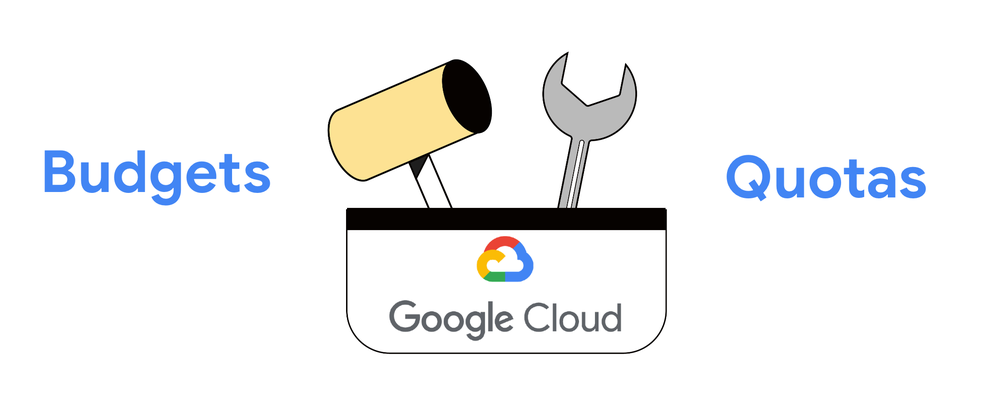
Budgets and custom quotas are two powerful tools provided by Google Cloud that you can (and I’d argue you should!) use to manage BigQuery costs. So let’s dive into how each of these work and help you get started.
Budgets
As your cloud usage grows and changes over time, your costs will change too. Budgets allow you to monitor all of your Google Cloud charges in one place, including BigQuery. They can track both your actual and forecasted spend, and alert you when you’re exceeding your defined budgets, which helps you to both avoid unexpected expenses and plan for growth.
Budgets can be configured for a Cloud Billing account (that can include more than one project linked to the billing account), or for individual projects. To manage budgets for a Cloud Billing account, you need the Billing Account Administrator or Billing Account Costs Manager role on the Cloud Billing account. To manage budgets for an individual project, you need the Project Owner or Project Editor role on the project.
Budgets can be created within the Billing Console in the Budgets & alerts page. At a high-level, you will define the following areas when creating a budget:
ScopeBudgets are a tool that span Google Cloud, and you can scope budgets to apply to the spend in an entire Cloud Billing account, or narrow the scope by filtering on projects, services, or labels. To create a budget focused on BigQuery spend, you can scope it to the BigQuery service. Note that this scope includes both BigQuery on-demand query usage and BigQuery storage.Budget amountThe budget amount can be a total that you specify, or you can base the budget amount on the previous calendar period’s spend.ActionsAfter setting the budget amount, you can set multiple threshold rules to trigger email notifications. Each threshold can be customized as a percentage of the total budget amount, and can be based on actual costs (as you’re charged for using services) or forecasted costs (as Google Cloud forecasts that you’re going to be spending a certain amount). Using forecasted costs can alert you before you actually spend and stay ahead of any issues!
Screen capture of creating a budget in the Billing Console
You have several options for creating a budget: you can use the Cloud Console (as shown in the above screenshot), the gcloud command-line tool, or the Cloud Billing API.
Once your budget is in place, email alert notifications will be sent when you hit (or are forecasted to hit) your budget!
Monitoring spending with budgets
In addition to any of the alert actions you choose when setting up a budget, you can monitor your spending against your budgets using the Cloud Billing dashboard or the Budget API. You can see how much of your budget has been consumed, which resources are contributing the most to your costs, and where you might be able to optimize your usage.
Sample screen capture of of budget report
Tips for using budgets
Budget email alerts are sent to users who have Billing Account Administrator and Billing Account User roles by default. While this is a great first step, you can also configure budgets to notify users through Cloud Monitoring, or you can have regular budget updates sent to Pub/Sub for full customization over how you want to respond to budget updates such as sending messages to Slack.With the Cloud Billing Budget API, you can view, create, and manage budgets programmatically at scale. This is especially useful if you’re creating a large number of budgets across your organization.While this blog post focuses on using budgets for BigQuery usage, budgets are a tool that can be used across Google Cloud, so you can use this tool to manage Cloud spend as a whole or target budgets for particular services or projects.
Custom quota
Custom quotas are a powerful feature that allow you to set hard limits on specific resource usage. In the case of BigQuery, quotas allow you to control query usage (number of bytes processed) at a project- or user-level. Project-level custom quotas limit the aggregate usage of all users in that project, while user-level custom quotas are separately applied to each user or service account within a project.
Custom quotas are relevant when you are using BigQuery’s on-demand pricing model, which charges for the number of bytes processed by each query. When you are using the capacity pricing model, you are charged for compute capacity (measured in slots) used to run queries, so limiting the number of bytes processed is less useful.
By setting custom quotas, you can control the amount of query usage by different teams, applications, or users within your organization, preventing unexpected spikes in usage and costs.
Note that quotas are set within a project, and you must have the Owner, Editor, or Quota Administrator role on that project in order to set quotas.
Custom quota can be set by heading to the IAM & Admin page of the Cloud console, and then choosing Quotas. This page contains hundreds of various quota, so use the filter functionality with Metric: bigquery.googleapis.com/quota/query/usage to help you zero in on the two quota options for BigQuery query usage:
Query usage per day <- this is the project-level quotaQuery usage per user per day <- this is the user-level quota
Screen capture of the BigQuery usage quotas in the Cloud Console
After selecting one or both quotas, click toEdit Quotas. Here you will define your daily limits for each quota in tebibytes (TiB), so be sure to make any necessary conversions.
Screen capture of setting new custom quota amounts in the Cloud Console
To set custom quotas for BigQuery, you can use the Cloud Console (as described above), the gcloud command-line tool, or the Service Usage API. You can also monitor your quotas and usage within the Quotas page or using the Service Usage API.
Screen capture of monitoring quota usage within the Quota page of the Cloud Console
Tips for using custom quotas
You may use either project-level or user-level of these quota options, or both in tandem. Used in tandem, usage will count against both quotas, and adhere to the stricter of the two limits.Once quota is exceeded, the user will receive a usageQuotaExceeded error and the query will not execute. Quotas are proactive, meaning, for example, you can’t run an 11 TB query if you have a 10 TB quota.Daily quotas reset at midnight Pacific Time.Separate from setting a custom quota, you can also set a maximum bytes billed for a specific query (say, one you run on a schedule) to limit query costs.
Differences between budgets and custom quotas
Now that you’ve learned more about budgets and custom quota, let’s look at them side-by-side and note some of their differences:
Their scope: Budgets are tied to a billing account (which can be shared across projects), while quotas are set for individual projects.What they track: Budgets are set for a specific cost amount, while quotas are set for specific resource or service usage.How they are enforced: Budgets track your costs and alert you when you’re exceeding your budget, while quotas enforce a hard limit on the amount of resources that can be used in a project and will return an error when a user/service tries to exceed the limit.
Next steps
Tracking and analyzing your BigQuery costs will make you feel more at ease when running queries within the on-demand pricing model, and it can help you make informed decisions, optimize your costs, and maximize the value of your cloud spend.
As you scale your BigQuery environment, you may want to move your workloads to the BigQuery editions pricing model, which charges by the amount of capacity allocated to your workload, measured in slots (a unit of measure for BigQuery compute power) rather than per each query. This model also can provide discounted capacity for long term commitments. One of BigQuery’s unique features is the ability to combine the two different pricing models (on-demand and capacity) to optimize your costs.
You can get started with budgets and quota using the in-console walkthroughs I mentioned earlier for creating budgets or setting custom quota. And head to our Cost Management page to learn about more features to help you monitor, control, and optimize your cloud costs.
Google Cloud BigQuery is a key service that helps you create a Data Warehouse that provides the scale and ease of querying large data sets. Let’s say that you have standardized on using BigQuery and have set up data pipelines to maintain the datasets. The next question would be to determine how best to make this data available to applications. APIs are often the way forward for this and what I was looking to experiment with is to consider a service that helps me create an API around my data sources (BigQuery in this case) and do it easily.
In this blog post, we shall see how to use Hasura, an open-source solution, that helped me create an API around my BigQuery dataset.
The reason to go with Hasura is the ease with which you can expose your domain data via an API. Hasura supports a variety of data sources including BigQuery, Google Cloud SQL and AlloyDB. You control the model, relationships, validation and authorization logic through metadata configuration. Hasura consumes this metadata to generate your GraphQL and REST APIs. It’s a low-code data to API experience, without compromising any of the flexibility, performance or security you need in your data API.
While Hasura is open-source, it also has fully managed offerings on various cloud providers including Google Cloud.
Pre-requisites
You need to have a Google Cloud Project. Do note down the Project Id of the project since we will need to use that later in the configuration in Hasura.
BigQuery dataset – Google Trends dataset
Our final goal is to have a GraphQL API around our BigQuery dataset. So what we need to have in place is a BigQuery dataset. I have chosen the Google Trends database that is made available in the Public Datasets program in BigQuery. This is an interesting dataset that makes available (both US and Internationally), the top 25 overall or top 25 rising queries from Google Trends from the past 30 days.
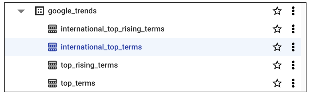
I have created a sample dataset in BigQuery in my Google Cloud project named ‘google_trends’ and have copied the dataset and the tables from the bigquery-public-data dataset. The tables are shown below:
Google Trends dataset
What we are interested in is the international_top_terms that helps me to see the trends across countries that are supported in the Google Trends dataset that has been made available.
The schema for the international_top_terms dataset schema is shown below:
International Top Terms table schema
A sample BigQuery query (Search terms from the previous day in India) that we eventually would like to expose over the GraphQL API is shown below:
If I run this query in the BigQuery workspace, I get the following result (screenshot below):
International Trends sample data
Great ! This is all we need for now from a BigQuery point of view. Remember you are free to use your own dataset if you’d like.
Service account
We will come to the Hasura configuration in a while, but before that, do note that the integration between Hasura and Google Cloud will require that we generate a service account with the right permissions. We will provide that service account to Hasura, so that it can invoke the correct operations on BigQuery to configure and retrieve the results.
Service account creation in Google Cloud is straightforward and you can do that from the Google Cloud Console → IAM and Admin menu option.
Create a Service account with a name and description.
Service Account Creation
In the permissions for the service account, ensure that you have the following Google Cloud permissions, specific to BigQuery:
Service Account Permissions
Once the service account is created, you will need to export this account via its credentials (JSON) file. Keep that file safely as we will need that in the next section.
This completes the Google Cloud part of the configuration.
Hasura configuration
You need to sign up with Hasura as a first step. Once you have signed it, click on New Project and then choose the Free Tier and Google Cloud to host the Hasura API Layer, as shown below. You will also need to select the Google Cloud region to host the Hasura service in and then click on the Create Project button.
Hasura Project Creation
Setting up the data connection
Once the project is created, you need to establish the connectivity between Hasura and Google Cloud and specifically in this case, set up the Data Source that Hasura needs to configure and talk to.
For this, visit the Data section as shown below. This will show that currently there are no databases configured i.e. Databases(0). Click on the Connect Database button.
Hasura Data Source creation
From the list of options available, select BigQuery and then click on Connect Existing Database.
Hasura BigQuery Data Source creation
This will bring up a configuration screen (not shown here), where you will need to entire the service account, Google Project Id and BigQuery Dataset name.
Create an environment variable in the Hasura Settings that contains your Service Account Key (JSON file contents). A sample screenshot from my Hasura Project Settings is shown below. Note that the SERVICE_ACCOUNT_KEY variable below has the value of the JSON Key contents.
Hasura Project Settings
Coming back to the Database Connection configuration, you will see a screen as shown below. Fill out the Project Id and Dataset value accordingly.
Hasura BigQuery Datasource configuration
Once the data connection is successfully set up, you can now mark which tables need to be tracked. Go to the Datasource settings and you will see that Hasura queried the metadata to find the tables in the dataset. You will see the tables listed as shown below:
Hasura BigQuery Datasource tables
We select the table that we are interested in tracking i.e. select it and then click on the Track button.
Hasura BigQuery Datasource table tracking
This will mark the table as tracked and we will now be able to go to the GraphQL Test UI to test out the queries.
The API tab provides us with a nice Explorer UI where you can build out the GraphQL query in an intuitive manner.
Enterprises are generating data at an exponential rate, spanning traditional structur transactional data, semi-structured data like JSON and unstructured data like images and audio. The diversity and volume of data presents complex architectural challenges for data processing, data storage and query engines, requiring developers to build custom transformation pipelines to deal with semi-structured and unstructured data.
In this post we will explore the architectural concepts that power BigQuery’s support for semi-structured JSON, which eliminates the need for complex preprocessing and provides schema flexibility, intuitive querying and the scalability benefits afforded to structured data. We will review the storage format optimizations, performance benefits afforded by the architecture and finally discuss how they affect the billing for queries that use JSON paths.
Integration with the Capacitor File Format
Capacitor, a columnar storage format, is the backbone of BigQuery’s underlying storage architecture. Based on over a decade of research and optimization, this format stores exabytes of data, serving millions of queries. Capacitor is optimized for storing structured data. Capacitor uses techniques like Dictionary, Run Length Encoding (RLE), Delta encoding etc. to store the column values optimally. To maximize RLE, it also employs record-reordering. Usually, row order in the table does not have significance, so Capacitor is free to permute rows to
improve RLE effectiveness. Columnar storage lends itself to block oriented vectorized processing which is employed by an embedded expression library.
To natively support semi-structured formats like JSON, we developed the next generation of the BigQuery Capacitor format optimized for sparse semi-structured data.
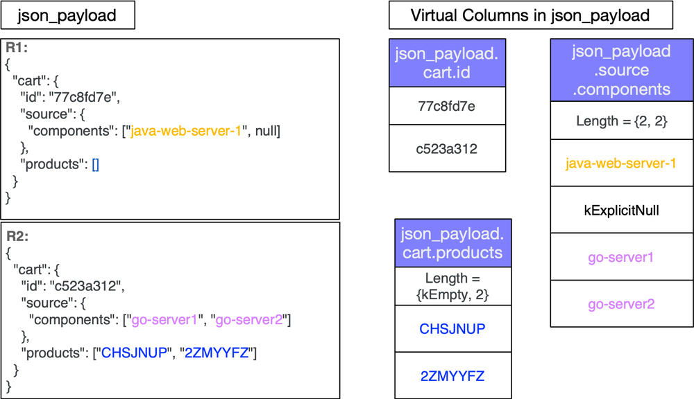
On ingestion, JSON data is shredded into virtual columns to the extent possible. JSON keys are typically only written once per column instead of once per row. Other non data characters such as colons and whitespace are not part of the data stored in the columns. Placing the values in columns allows us to apply the same encodings that are used for structured data such as Dictionary encoding, Run Length Encoding and Delta encoding. This greatly reduces storage and thus IO costs at query time. Additionally, JSON nulls and arrays are natively understood by the format leading to optimal storage of virtual columns. Fig. 1 shows the virtual columns for records R1 and R2. The records are fully shredded into nested columns.
Figure 1: Shows the virtual columns for given records R1 and R2
BigQuery’s native JSON data type maintains the nested structure of JSON by understanding JSON objects, arrays, scalar types, JSON nulls (‘null’) and empty arrays
Capacitor, the underlying file-format of the native JSON data type, uses record-reordering to keep similar data and types together. The objective of record-reordering is to find an optimal layout where Run Length Encoding across the rows is maximized resulting in smaller virtual columns. In the event of a particular key having different types, say integer and string across a range of rows in the file, record-reordering results in grouping the rows with the string data type together and the rows with the integer type together resulting in run length encoded spans of missing values in both virtual columns thus producing smaller columns. To illustrate the column sizes, Fig. 2 shows a single key `source_id` that is either an integer or a string across the source JSON data. This produces two virtual columns based on the types. It showcases how reordering and applying RLE results in small virtual columns. For simplicity, we use `kMissing` to denote a missing value.
Figure 2 : Shows the effect of row reordering on column sizes.
Capacitor was specifically designed to handle well structured datasets. This was challenging for JSON data which takes a variety of shapes with a mix of types. Here are some of the challenges that we overcame while building the next generation of Capacitor that natively supported the JSON data type.
Adding/Removing keys JSON keys are treated as optional elements thus marking them as missing in the rows that don’t have the keys.Changing Scalar Types Keys that change scalar types such as string, int, bool and float across rows are written into distinct virtual columns.Changing Types with non-scalar types For non-scalar values such as object and array, the values are stored in an optimized binary format that’s efficient to parse.
At ingestion time, after shredding the JSON data into virtual columns, the logical size of each virtual column is calculated based on the data size [https://cloud.google.com/bigquery/docs/reference/standard-sql/data-types#data_type_sizes] for specific types such as INT64, STRING, BOOL. Thus the size of the entire JSON column is the sum of the data sizes of each virtual column stored in it. This cumulative size is stored in metadata and becomes the upper bound logical estimated size when any query touches the JSON column.
These techniques produce individual virtual columns that are substantially smaller when compared to the original JSON data. For example, storing a migrated version of bigquery-public-data.hacker_news.full discussed below as a JSON column compared to STRING, leads to a direct saving of 25% for logical uncompressed bytes.
Improved Query Performance with JSON native data types
With the JSON data stored in a STRING column, if you wanted to filter on certain JSON paths or only project specific paths, the entire JSON STRING row would have to be loaded from storage, decompressed and then each filter and projection expression evaluated one row at a time.
In contrast, with the native JSON data type, only the necessary virtual columns are processed by BigQuery. To make projections and filter operations as efficient as possible, we added support for compute and filter pushdown of JSON operations. Projections and filter operations are pushed down to the embedded evaluation layer that can perform the operations in a vectorized manner over the virtual columns making these very efficient in comparison to the STRING type.
When the query is run, customers are only charged based on the size of the virtual columns that were scanned to return the JSON paths requested in the SQL query. For example, in the query shown below, if payload is a JSON column with keys `reference_id` and `id`, only the specific virtual columns representing the JSON keys namely `reference_id` and `id` are scanned across the data.
code_block<ListValue: [StructValue([(‘code’, ‘SELECT payload.reference_id FROM tablernWHERE Safe.INT64(payload.id) = 21’), (‘language’, ”), (‘caption’, <wagtail.rich_text.RichText object at 0x3ee5ea1a7610>)])]>
Note: The estimate always shows the upper bound of the total JSON size rather than specific information about the virtual columns being queried.
With the JSON type, on-demand billing reflects the number of logical bytes that had to be scanned. Since each virtual column has a native data type such as INT64, FLOAT, STRING, BOOL, the data size calculation is a summation of sizes of each column `reference_id` and `id` that was scanned and follows the standard bigquery data type size [https://cloud.google.com/bigquery/docs/reference/standard-sql/data-types#data_type_sizes]
With BigQuery Editions, optimized virtual columns lend to queries that require far less IO and CPU in comparison to storing the JSON string unchanged since you’re scanning specific columns rather than loading the entire JSON blob and extracting the paths from the JSON string.
With the new type, BigQuery is now able to process just the paths within the JSON that are requested by the SQL query. This can substantially reduce query cost.
For instance running a query to project a few fields such as `$.id` and `$.parent` from a migrated version of the public dataset `biquery-public-data.hacker_news.full` containing both STRING and JSON type of the same data shows a reduction of processed bytes from 18.28GB to 514MB which is a 97% reduction.
The following query was used for creating a table from the public dataset that contains both a STRING column in `str_payload` and a JSON column in `json_payload` and saved to a destination table.
code_block<ListValue: [StructValue([(‘code’, ‘– Saved to a –destination_table my_project.hacker_news_json_strrnSELECT TO_JSON(t) AS json_payload, TO_JSON_STRING(t) AS str_payload FROM `bigquery-public-data.hacker_news.full` trnrn– Processed bytes for `str_payload.id` 18.28 GBrnSELECT JSON_QUERY(str_payload, “$.id”) FROM `my_project.hacker_news_json_and_str`rnWHERE JSON_VALUE(str_payload, “$.parent”) = “11787862” rnrnrn– processed bytes for `json_payload.id` 514 MBrnSELECT json_payload.id FROM `my_project.hacker_news_json_str`rnWHERE LAX_INT64(json_payload.parent) = 11787862’), (‘language’, ”), (‘caption’, <wagtail.rich_text.RichText object at 0x3ee5ea1a7310>)])]>
Summary
The improvements to the Capacitor file format have enabled the flexibility required by today’s semi-structured data workloads. Shredding the JSON data into virtual columns along with enhancements such as compute and filter pushdown has shown promising results. Since the JSON data is shredded, only the virtual columns matching the requested JSON paths are scanned by BigQuery. Compute and filter pushdowns make it possible for the runtime to do work closest to the data evaluation layer in a vectorized manner thus exhibiting better performance. Lastly these choices have made it possible to improve compression and reduce the IO/CPU usage (smaller columns = less IO) as a result, reducing the slot usage for fixed-rate reservations and the bytes billed for on-demand usage.
Beyond the storage and query optimizations, we’ve also invested in programmability and ease of use by providing a range of JSON SQL Functions. Also see the latest blog post about the new JSON SQL functions that were released recently.
Next Steps
Convert to the JSON native data type in BigQuery today!
To convert your table with a STRING JSON column into a table with a native JSON column, run the following query and save the results to a new table, or select a destination table.
code_block<ListValue: [StructValue([(‘code’, ‘SELECT * EXCEPT (payload), SAFE.PARSE_JSON (payload) as json_payloadrnFROM <table>’), (‘language’, ”), (‘caption’, <wagtail.rich_text.RichText object at 0x3ee5ea1a7a90>)])]>
Looker Studio supports self-serve analytics for ad hoc data, and together with Looker, contributes to the more than 10 million users who access the Looker family of products each month. Today, we are introducing new ways for analysts to provide business users with options to explore data and self-serve business decisions, expanding ways all our users can analyze and explore data — leading to faster and more informed decisions.
Introducing personal report links
Business users often leverage shared dashboards from data analysts, which contain key company metrics and KPIs, as a starting point and want to explore beyond the curated analysis to arrive at more specific insights for their own data needs. The introduction of personal reports in Looker Studio enables this activity, delivering a private sandbox for exploration so users can self-serve their own questions and find insights faster – without modifying the original curated report.
Whether you share a report link in group chats or direct messages, an individual copy is created for each user that opens it so that everyone gets their own personal report.
Personal Looker Studio reports are designed to be ephemeral, meaning you don’t need to worry about creating unwanted content, but if you land on valuable insights that you want to keep, you can save and share these reports with new links, separate from the original report you built from.
You can learn more about how personal reports work and how to use them in our Help Center.
Looker Studio Personal Link Visual
Automated report updates
Your analysis and insights are only as good as the freshness of your reports. Looker Studio users can now enable their reports to auto-refresh data at a predefined cadence, so critical business decisions are based on current and updated information.
To learn more about how auto-refresh works, including details on how it works with cache, presentation mode, and existing data freshness settings, visit our Help Center.
Looker Studio Auto refresh feature Visual
Faster filtering in reports
Quick filters enable powerful exploration to slice data and uncover hidden patterns and insights within the context of your report. Quick filters don’t affect other users’ views, so whether you are exploring in a shared or personal report, your unique view is only shared once you are ready. The filter bar also gives you a complete picture of whether applied filters originate from interactive cross-chart filtering or quick filters.
Learn more about how to add quick filters in reports in our Help Center.
Looker Studio Quick filters and filter bar feature Visual
Pause updates
Configuring multiple filters and charts for exploration can quickly add to the query volume, even with presence of a cache. We’ve heard from analysts that they want better control over running queries, so they can optimize query volume and, thus, query costs.
We have added the ability to pause updates, giving you the flexibility to fully configure chart elements like fields, filters, parameters, sorting, and calculated formulas before running any data updates. You can then simply resume updates to see the updated data. Pausing updates does not prevent any style changes, so you can continue to modify design elements and other detailed styles and formatting without running a single query. Learn more about this feature in our Help Center.
The new pause report updates feature in Looker Studio has meaningfully improved the report creation experience. Asset producers can build and test reports without wasting database resourcing waiting for data to reload. Caroline Bollinger BI Tooling Product, Wayfair
View underlying data
Data accuracy is one thing — being able to see its detail is another. As analysts configure charts to build reports and design information hierarchy, previewing the underlying data is important for understanding context and seeing what data is available and its structure so you can make the best decisions about what to include in your analysis. It’s also handy when troubleshooting or customizing your reports.
This feature allows analysts to preview all the data that appears in a chart, including the primary dimensions, breakdown dimensions, and metrics. Learn more about how to view underlying data in our Help Center.
Looker Studio Data preview feature Visual
With this collection of updates, Looker Studio users can now easily know the data they share is up-to-date, inspect it in detail, rapidly create filters, and share personal links to reports. The goal remains, as always, to empower users to make smart and impactful decisions based on their enterprise data. To stay on top of all our latest features, view our release notes. Access Looker Studio for free and learn more about Looker Studio Pro.
Geographical redundancy is one of the keys to designing a resilient data lake architecture in the cloud. Some of the use cases for customers to replicate data geographically are to provide for low-latency reads (where data is closer to end users), comply with regulatory requirements, colocate data with other services, and maintain data redundancy for mission-critical apps.
BigQuery already stores copies of your data in two different Google Cloud zones within a dataset region. In all regions, replication between zones uses synchronous dual writes. This ensures in the event of either a soft (power failure, network partition) or hard (flood, earthquake, hurricane) zonal failure, no data loss is expected, and you will be back up and running almost immediately.
We are excited to take this a step further with the preview of cross-region dataset replication, which allows you to easily replicate any dataset, including ongoing changes, across cloud regions. In addition to ongoing replication use cases, you can use cross-region replication to migrate BigQuery datasets from one source region to another destination region.
How does it work?
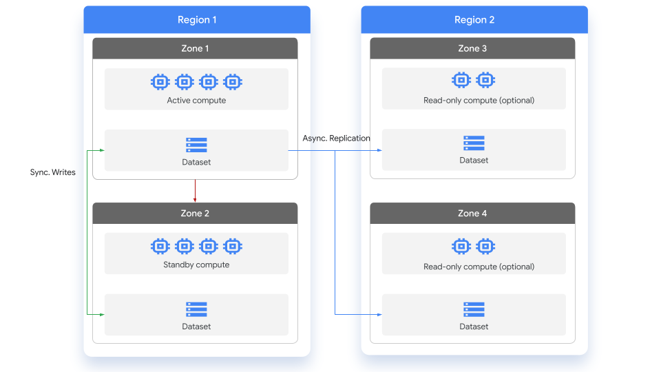
BigQuery provides a primary and secondary configuration for replication across regions:
Primary region: When you create a dataset, BigQuery designates the selected region as the location of the primary replica.Secondary region: When you add a dataset replica in a selected region, BigQuery designates this as a secondary replica. The secondary region could be a region of your choice. You can have more than one secondary replica.
The primary replica is writeable, and the secondary replica is read-only. Writes to the primary replica are asynchronously replicated to the secondary replica. Within each region, the data is stored redundantly in two zones. Network traffic never leaves the Google Cloud network.
While replicas are in different regions, they do not have different names. This means that your queries do not need to change when referencing a replica in a different region.
The following diagram shows the replication that occurs when a dataset is replicated:
Replication in action
The following workflow shows how you can set up replication for your BigQuery datasets.
You can add a single replica to any dataset within each region or multi-region. After you add a replica, it takes time for the initial copy operation to complete. You can still run queries referencing the primary replica while the data is being replicated, with no reduction in query processing capacity.
code_block<ListValue: [StructValue([(‘code’, “– Create the primary replica in the primary region.rnCREATE SCHEMA my_dataset OPTIONS(location=’us-west1′);rnrn– Create a replica in the secondary region.rnALTER SCHEMA my_datasetrnADD REPLICA `us-east1`rnOPTIONS(location=’us-east1′);”), (‘language’, ”), (‘caption’, <wagtail.rich_text.RichText object at 0x3e0c6f3269d0>)])]>
To confirm the status that the secondary replica has successfully been created, you can query the creation_complete column in the INFORMATION_SCHEMA.SCHEMATA_REPLICAS view.
code_block<ListValue: [StructValue([(‘code’, “– Check the status of the replica in the secondary region.rnSELECT creation_time, schema_name, replica_name, creation_completernFROM `region-us-west1`.INFORMATION_SCHEMA.SCHEMATA_REPLICASrnWHERE schema_name = ‘my_dataset’;”), (‘language’, ”), (‘caption’, <wagtail.rich_text.RichText object at 0x3e0c6f326580>)])]>
Query the secondary replica
Once initial creation is complete, you can run read-only queries against a secondary replica. To do so, set the job location to the secondary region in query settings or the BigQuery API. If you do not specify a location, BigQuery automatically routes your queries to the location of the primary replica.
code_block<ListValue: [StructValue([(‘code’, ‘– Query the data in the secondary region..rnSELECT COUNT(*) rnFROM my_dataset.my_table;’), (‘language’, ”), (‘caption’, <wagtail.rich_text.RichText object at 0x3e0c6f326460>)])]>
If you are using BigQuery’s capacity reservations, you will need to have a reservation in the location of the secondary replica. Otherwise, your queries will use BigQuery’s on-demand processing model.
Promote the secondary replica as primary
To promote a replica to be the primary replica, use the ALTER SCHEMA SET OPTIONS DDL statement and set the primary_replica option. You must explicitly set the job location to the secondary region in query settings.
code_block<ListValue: [StructValue([(‘code’, “ALTER SCHEMA my_dataset SET OPTIONS(primary_replica = ‘us-east1’)”), (‘language’, ”), (‘caption’, <wagtail.rich_text.RichText object at 0x3e0c6f3262b0>)])]>
After a few seconds, the secondary replica becomes primary, and you can run both read and write operations in the new location. Similarly, the primary replica becomes secondary and only supports read operations.
Remove a dataset replica
To remove a replica and stop replicating the dataset, use the ALTER SCHEMA DROP REPLICA DDL statement. If you are using replication for migration from one region to another region, delete the replica after promoting the secondary to primary. This step is not required, but is useful if you don’t need a dataset replica beyond your migration needs.
code_block<ListValue: [StructValue([(‘code’, ‘ALTER SCHEMA my_datasetrnDROP REPLICA IF EXISTS `us-west1`;’), (‘language’, ”), (‘caption’, <wagtail.rich_text.RichText object at 0x3e0c6f3260a0>)])]>
Getting started
We are super excited to make the preview for cross-region replication available for BigQuery, which will allow you to enhance your geo-redundancy and support region migration use cases. Looking ahead, we will include a console-based user interface for configuring and managing replicas. We will also offer a cross-region disaster recovery (DR) feature that extends cross-region replication to protect your workloads in the rare case of a total regional outage. You can also learn more about BigQuery and cross-region replication in the BigQuery cross-region dataset replication QuickStart.