Category Data Analytics

IBM mainframes have been around since the 1950s and are still vital for many organizations. In recent years many companies that rely on mainframes have been working towards migrating to the cloud. This is motivated by the need to stay relevant, the increasing shortage of mainframe experts and the cost savings offered by cloud solutions. 

One of the main challenges in migrating from the mainframe has always been moving data to the cloud. The good thing is that Google has open sourced a bigquery-zos-mainframe connector that makes this task almost effortless.

What is the Mainframe Connector for BigQuery and Cloud Storage?

The Mainframe Connector enables Google Cloud users to upload data to Cloud Storage and submit BigQuery jobs from mainframe-based batch jobs defined by job control language (JCL). The included shell interpreter and JVM-based implementations of gsutil and bq command-line utilities make it possible to manage a complete ELT pipeline entirely from z/OS. 

This tool moves data located on a mainframe in and out of Cloud Storage and BigQuery; it also transcodes datasets directly to ORC (a BigQuery supported format). Furthermore, it allows users to execute BigQuery jobs from JCL, therefore enabling mainframe jobs to leverage some of Google Cloud’s most powerful services.

The connector has been tested with flat files created by IBM DB2 EXPORT that contain binary-integer, packed-decimal and EBCDIC character fields that can be easily represented by a copybook. Customers with VSAM files may use IDCAMS REPRO to export to flat files, which can then be uploaded using this tool. Note that transcoding to ORC requires a copybook and all records must have the same layout. If there is a variable layout, transcoding won’t work, but it is still possible to upload a simple binary copy of the dataset.

Using the bigquery-zos-mainframe-connector

A typical flow for Mainframe Connector involves the following steps:

Reading the mainframe datasetTranscoding the dataset to ORCUploading ORC to Cloud StorageRegistering it as an external tableRunning a MERGE DML statement to load new incremental data into the target table

Note that if the dataset does not require further modifications after loading, then loading into a native table is a better option than loading into an external table.

In regards to step 2, it is important to mention that DB2 exports are written to sequential datasets on the mainframe and the connector uses the dataset’s copybook to transcode it to an ORC.

The following simplified example shows how to read a dataset on a mainframe, transcode it to ORC format, copy the ORC file to Cloud Storage, load it to a BigQuery-native table and run SQL that is executed against that table.

1. Check out and compile:

2. Upload the assembly jar that was just created in target/scala-2.13 to a path on your mainframe’s unix filesystem.

3. Install the BQSH JCL Procedure to any mainframe-partitioned data set you want to use as a PROCLIB. Edit the procedure to update the Java classpath with the unix filesystem path where you uploaded the assembly jar. You can edit the procedure to set any site-specific environment variables.

4. Create a job

STEP 1:

This step reads the dataset from the INFILE DD and reads the record layout from the COPYBOOK DD. The input dataset could be a flat file exported from IBM DB2 or from a VSAM file. Records read from the input dataset are written to the ORC file at gs://bucket/my_table.orc with the number of partitions determined by the amount of data.

STEP 2:

This step submits a BigQuery load job that will load ORC file partitions from my_table.orc into MY_DATASET.MY_TABLE. Note this is the path that was written to on the previous step. 

STEP 3:

This step submits a BigQuery Query Job to execute SQL DML read from the QUERY DD (a format FB file with LRECL 80). Typically the query will be a MERGE or SELECT INTO DML statement that results in transformation of a BigQuery table. Note: the connector will log job metrics but will not write query results to a file.

Running outside of the mainframe to save MIPS

When scheduling production-level load with many large transfers, processor usage may become a concern. The Mainframe Connector executes within a JVM process and thus should utilize zIIP processors by default, but if capacity is exhausted, usage may spill over to general purpose processors. Because transcoding z/OS records and writing ORC file partitions requires a non-negligible amount of processing, the Mainframe Connector includes a gRPC server designed to handle compute-intensive operations on a cloud server; the process running on z/OS only needs to upload the dataset to Cloud Storage and make an RPC call. Transitioning between local and remote execution requires only an environment variable change. Detailed information on this functionality can be found here. 

Acknowledgements
Thanks to those who tested, debugged, maintained and enhanced the tool: Timothy Manuel, Suresh Balakrishnan,Viktor Fedinchuk,Pavlo Kravets

When deploying models to the Vertex AI prediction service, each model is by default deployed to its own VM. To make hosting more cost effective, we’re excited to introduce model co-hosting in public preview, which allows you to host multiple models on the same VM, resulting in better utilization of memory and computational resources. The number of models you choose to deploy to the same VM will depend on model sizes and traffic patterns, but this feature is particularly useful for scenarios where you have many deployed models with sparse traffic.

Understanding the Deployment Resource Pool

Co-hosting model support introduces the concept of a Deployment Resource Pool, which groups together models to share resources within a VM. Models can share a VM if they share an endpoint, but also if they are deployed to different endpoints. 

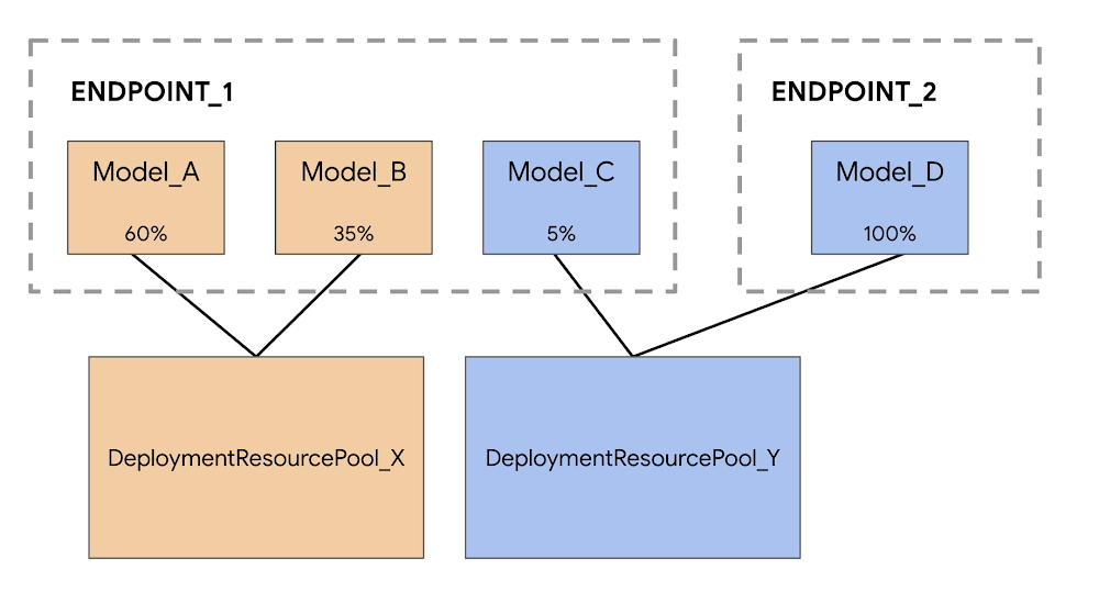
For example, let’s say you have four models and two endpoints, as shown in the image below.

Model_A, Model_B, and Model_C are all deployed to Endpoint_1 with traffic split between them. And Model_D is deployed to Endpoint_2, receiving 100% of the traffic for that endpoint. 

Instead of having each model assigned to a separate VM, we can group Model_A and Model_B to share a VM, making them part of DeploymentResourcePool_X. We can also group models that are not on the same endpoint, so Model_C and Model_D can be hosted together in DeploymentResourcePool_Y. 

Note that for this first release, models in the same resource pool must also have the same container image and version of the Vertex AI pre-built TensorFlow prediction containers. Other model frameworks and custom containers are not yet supported.

Co-hosting models with Vertex AI Predictions

You can set up model co-hosting in a few steps. The main difference is that you’ll first create a DeploymentResourcePool, and then deploy your model within that pool. 

Step 1: Create a DeploymentResourcePool

You can create a DeploymentResourcePool with the following command. There’s no cost associated with this resource until the first model is deployed.

Step 2: Create a model

Models can be imported to the Vertex AI Model Registry at the end of a custom training job, or you can upload them separately if the model artifacts are saved to a Cloud Storage bucket. You can upload a model through the UI or with the SDK using the following command:

When the model is uploaded, you’ll see it in the model registry. Note that the deployment status is empty since the model hasn’t been deployed yet.

Step 3: Create an endpoint

Next, create an endpoint via the SDK or the UI. Note that this is different from deploying a model to an endpoint.

endpoint = aiplatform.Endpoint.create(‘cohost-endpoint’)

When your endpoint is created, you’ll be able to see it in the console.

Step 4: Deploy Model in a Deployment Resource Pool

The last step before getting predictions is to deploy the model within the DeploymentResourcePool you created.

When the model is deployed, you’ll see it ready in the console. You can deploy additional models to this same DeploymentResourcePool for co-hosting using the same endpoint we created already, or using a new endpoint.

Step 5: Get a prediction

Once the model is deployed, you can call your endpoint in the same way you’re used to.

x_test= [‘The movie was spectacular. Best acting I’ve seen in a long time and a great cast. I would definitely recommend this movie to my friends!’]
endpoint.predict(instances=x_test)

What’s next

You now know the basics of how to co-host models on the same VM. For an end to end example, check out this codelab, or refer to the docs for more details. Now it’s time for you to start deploying some models of your own!

After migrating databases to Google Cloud,  Cloud SQL developers and business users can use familiar business intelligence tools and services like Microsoft Power BI to connect to and report from Cloud SQL MySQL, PostgreSQL, and SQL Server databases.  

The ability to quickly migrate databases to GCP without having to worry about refactoring or developing new reporting and BI tools is a key capability for businesses migrating to CloudSQL. Organizations can migrate today, and then replatform databases and refactor reporting in subsequent project phases.

The following guide demonstrates key steps to configure Power BI reporting from Cloud SQL. While your environment and requirements may vary, the design remains the same. 

To begin, create three Cloud SQL Instances, each with a Private IP address.

After creating the database instances, create a Windows VM in the same VPC as the Cloud SQL instances. Install and configure the Power BI Gateway on this VM along with the required ODBC connectors.

Download and Install ODBC Connectors for PostgreSQL and MySQL.

Postgres:  https://www.postgresql.org/ftp/odbc/versions/msi/  

MySQL: https://dev.mysql.com/downloads/connector/odbc/ 

 Configure System DSNs for each Database connection. Examples follow. 

SQL Server

PostgreSQL

MySQL

The traffic between the CloudSQL instance and the VM hosting the data gateway stays inside the Google VPC and is encrypted via Encryption in Transit in Google Cloud. To add an additional layer of SSL encryption for the data inside the Google VPC, configure each System DSN to use CloudSQL SSL/TLS certificates . 

Next, download, install, and configure the Power BI Gateway. Note that the gateway may be installed in an HA configuration. The screenshot below shows a single standalone gateway. 

On-premises data gateway configuration: Create a new on-premises data gateway

On-premises data gateway configuration: Validate Gateway Configuration

On-premises data gateway configuration: Review logging settings

On-premises data gateway configuration: Review HTTPS mode

Make sure that outgoing HTTPS traffic is allowed to exit from the VPC.

Next, download and open Power BI Desktop. Log into Power BI and select “Manage gateways” to configure data sources.

Add data sources for each instance, and then test the data source connections. In the example below a data source is added for each CloudSQL instance.

Load test data into each database instance (optional). In the example below a simple table containing demo data is created in each source database.

Launch Power BI desktop and log in. Next, add data sources and create a report. Select “Get data” and add ODBC connections for CloudSQL SQL Server, PostgreSQL and MySQL, then create a sample report with data from each instance.

Using the Power BI publish feature, publish the report to the Power BI service. Once the report and data sources are published, update the data sources in the Power BI workspace to point to the data gateway data sources.

Map the datasets to the CloudSQL database gateway connections.

Optional: Schedule a refresh time.

To perform an end-to-end test, update the test data and refresh the reports to view the changes.

Use the Publish to – Power BI Service to publish Power BI reports that were developed with Power BI Report Builder to a workspace (Power BI Premium Capacity is required).

Conclusion

Hopefully this blog was helpful in demonstrating how Power BI reports and dashboards can connect to Google Cloud SQL Databases using the Power BI Gateway. You can also use the Power BI Gateway to connect to your Big Query datasets and databases running on GCE VMs. For more information on Cloud SQL, please visit Google Cloud Platform Cloud SQL.  

Financial services institutions are increasingly aware of the significant role they can play in addressing climate change. As allocators of capital through their lending and investment portfolios, they direct financial resources for corporate development and operations in the wider economy. 

This capital allocation responsibility balances growth opportunities with risk assessments to optimize risk-adjusted returns. Identifying, analyzing, reporting, and monitoring climate risks associated with physical hazards, such as wildfires and water scarcity, is becoming an essential element of portfolio risk management.

Implementing a cloud-native portfolio climate risk analytics system

To help quantify these climate risks, this design pattern includes cloud-native building blocks that financial services institutions can use to implement a portfolio climate risk analytics system in their own environment. This pattern includes a sample dataset from RS Metrics and leverages several Google Cloud products, such as BigQuery, Data Studio, Vertex AI Workbench, and Cloud Run. The technical architecture is shown below.

Please refer to the source code repository for this pattern to get started, and read through the rest of this post to dig deeper into the underlying geospatial technology and business use cases in portfolio management. You can use the Terraform code provided in the repository to deploy the sample datasets and application components in your selected Google Cloud Project. The README has step-by-step instructions.

After deploying the technical assets, we recommend performing the following steps to get more familiar with the pattern’s technical capabilities:

Review the example Data Studio dashboard to get familiar with the dataset and portfolio risk analytics (see screenshot below)

Explore the included R Shiny app, deployed with Cloud Run, for more in-depth analytics

Visit Vertex AI Workbench and walk through the exploratory data analysis provided in the included Python-based Jupyter notebook

Drop into BigQuery to directly query the sample data for this pattern

The importance of granular objective data

Assessing exposure to climate risks under various climate change scenarios can involve combining geospatial layers, expertise in climate models, and using information about company operations. Depending on where they are located, companies’ physical assets – like their manufacturing facilities or office buildings – can be susceptible to varying types of climate risk. A facility located in a desert will likely experience greater water stress, and a plant located near sea level will have a larger risk of coastal flooding.

Asset-level physical climate risk analysis

Google Cloud partner RS Metrics offers two data products that cover a broad set of investable public equities: ESGSignals® and AssetTracker®. These products include 50 transition and physical climate risk metrics such as biodiversity, greenhouse gas (GHG) emissions, water stress, land usage, and physical climate risks. As an introduction to these concepts, we’ll first describe two key physical risks: water stress risk and fire risk.

Water Stress Risk

Water stress occurs when an asset’s demand for water exceeds the amount of water available for that asset, resulting in higher water costs or in extreme cases, complete loss of water supply. This can negatively impact the unit economics of the asset, or even result in the asset being shut down. According to a 2020 report from CDP, 357 surveyed companies disclosed a combined $301 billion in potential financial impact of water risks.

When investors don’t have asset location data, they use industry average water intensity and basin level water risk to estimate water stress risk, as described in a 2020 report by Ceres. However, ESGSignals® allows a more granular approach, integrating meteorological and hydrological variables at the basin and sub-basin levels, drought severity, evapotranspiration, and surface water availability for millions of individual assets.

As an example, let’s look at mining, a very water-intensive industry. One mining asset, the Cerro Colorado copper mine in Chile, produced 71,700 metric tons of copper in 2019, according to an open dataset published by Chile’s Ministry of Mining. ESGSignals® identifies this mining asset as having significant water stress, resulting in a water risk score of 75 out of 100. For assets like these, reducing water consumption via efficiency improvements and the use of desalinated seawater will not only save precious water resources for nearby communities, but also reduce operating costs over time.

Fire Risk

Wildfires have caused significant damage in recent years. For example, economists estimated that the 2019-2020 Australian bushfire season caused approximately A$103 billion in property damage and economic losses. Such wildfires pose safety and operational risk for all kinds of commercial operations located in Australia.

ESGSignals® fire risk score is calculated by combining historical fire events, proximity, and intensity of fire with company asset locations (AssetTracker®). Based on ESGSignals® assessments, the majority of mining assets located in Australia have medium to high exposure to fire risk.

Incorporating asset-level climate risk analytics into portfolio management 

Now that we have an understanding of the mechanics of asset-level climate risk, let’s focus on how portfolio managers could incorporate these analytics into their portfolio management processes, including portfolio selection, portfolio monitoring, and company engagement.

Portfolio selection

Portfolio selection can involve various investment tools. In screening, the portfolio manager sets up filtering criteria to select companies for inclusion in, or exclusion from, the portfolio. Asset-level climate risk scores can be included in these screening criteria, along with other financial or non-financial factors. 

For example, a portfolio manager could search for companies whose average asset-level water stress score is less than 30. This would result in an investment portfolio that has an overall lower risk from water stress than a given benchmark index (see figure below).

Portfolio monitoring

For portfolio monitoring, it’s important to first establish a baseline of physical climate risk for existing holdings within the portfolio. A periodic reporting process that looks for changes in water stress, wildfire, or other physical climate risk metrics can then be created. Any material changes in risk scores would trigger a more detailed analysis to determine the next best action, such as rebalancing the portfolio to meet the target risk profile.

Portfolio engagement

Some portfolio managers engage with companies held in their portfolios, either through shareholder initiatives or by meeting with corporate investor relations teams. For these investors, it’s important to clearly identify the assets with significant exposure to climate risks. 

To focus on the locations with the highest opportunity for impact, a portfolio manager could sort the millions of AssetTracker locations by water stress or fire risk score, and engage with companies near the top of these ranked lists. Highlighting mitigation opportunities for these most at-risk assets would be an effective engagement prioritization strategy.

Expanding beyond portfolio management

Applying an asset-level approach to physical climate risk analytics can be helpful beyond the use cases in portfolio management presented above. For example, risk managers in commercial banking could use this methodology to quantify lending risk during underwriting and ongoing loan valuation. Insurance companies could also use these techniques to improve risk assessment and pricing decisions for both new and existing policyholders.

To enable further insights, additional geospatial datasets can be blended with those used in this pattern via BigQuery’s geospatial analytics capabilities. Location information in these datasets, such as points or polygons encoded in a GEOGRAPHY data type, allow them to be combined together with spatial JOINs. For example, a risk analyst could join AssetTracker data with BigQuery public data, such as population information for states, counties, congressional districts, or zip codes available in the Census Bureau US Boundaries dataset.

A cloud-based data environment can help enterprises manage these and other sustainability analytics workflows. Infosys, a Google Cloud partner, provides blueprints and digital data intelligence assets to accelerate the realization of sustainability goals in a secure data collaboration space to connect, collect, correlate information assets such as RS Metrics geospatial data, enterprise data, and digital data to activate ESG intelligence within and across the financial value chain.

Curious to learn more? 

To learn more from RS Metrics about analyzing granular asset-level risk metrics with ESGSignals®, you can review their recent and upcoming webinars, or connect directly with them here.

To learn more about sustainability services from Infosys, reach out to the Infosys Sustainability team here. If you’d like a demo of the Infosys ESG Intelligence Cloud solution for Google Cloud, contact the Infosys Data, Analytics & AI team here.

To learn more about the latest strategies and tools that can help solve the tough challenges of climate change across industries, view the sessions on demand from our recent Google Cloud Sustainability Summit.

Special thanks to contributors
The authors would like to thank these Infosys collaborators: Manojkumar Nagdev, Rushiraj Pradeep Jaiswal, Padmaja Vaidyanathan, Anandakumar Kayamboo, Vinod Menon, and Rajan Padmanabhan. We would also like to thank Rashmi Bomiriya, Desi Stoeva, Connie Yaneva, and Randhika H from RS Metrics, and Arun Santhanagopalan, Shane Glass and David Sabater Dinter from Google.

Disclaimer
The information contained on this website is meant for the purposes of information only and is not intended to be investment, legal, tax or other advice, nor is it intended to be relied upon in making an investment or other decision. All content is provided with the understanding that the authors and publishers are not providing advice on legal, economic, investment or other professional issues and services.

Becoming Google Cloud certified has proven to improve individuals’ visibility within the job market, and demonstrate ability to drive meaningful change and transformation within organizations.  

1 in 4 Google Cloud certified individuals take on more responsibility or leadership roles at work, and  87% of Google Cloud certified users feel more confident in their cloud skills1.

75% of IT decision-makers are in need of technologically-skilled personnel to meet their organizational goals and close skill gaps2.

94% of those decision-makers agree that certified employees provide added value above and beyond the cost of certification3.

Prepare for certification with a no-cost learning opportunity

That’s powerful stuff, right?  That’s why we’ve teamed up with Coursera to support your journey to becoming Google Cloud certified.

As a new learner, get one month of no-cost access to your selected Google Cloud Professional Certificate on Coursera to help you prepare for the relevant Google Cloud certification exam. Choose from Professional Certificates in data engineering, cloud engineering, cloud architecture, security, networking, machine learning, DevOps and for business professionals, the Cloud Digital Leader.

Become Google Cloud certified

To  help you on your way to becoming Google Cloud certified, you can earn a discount voucher on the cost of the Google Cloud certification exam by completing the Professional Certificate on Coursera by August 31, 2022 

Simply visit our page on Coursera and start your one month no-cost learning journey today. 

Top tips to prepare for your Google Cloud certification exam

Get hands-on with Google Cloud
For those of you in a technical job role, we recommend leveraging the Google Cloud projects to build your hands-on experience with the Google Cloud console. With 500+ Google Cloud projectsnow available on Coursera, you can gain hands-on experience working in the real Google Cloud console, with no download or configuration required.

Review the exam guide
Exam guides provide the blueprint for developing exam questions and offer guidance to candidates studying for the exam. We´d encourage you to be prepared to answer questions on any topic in the exam guide, but it’s not guaranteed that every topic within an exam guide will be assessed.

Explore the sample questions
Taking a look at the sample questions on each certification page will help to familiarize you with the format of exam questions and example content that may be covered. 

Start your certification preparation journey today with a one month no-cost learning opportunity on Coursera. 

Want to know more about the value of Google Cloud Certification? Find out why IT leaders choose Google Cloud Certification for their teams.

1. Google Cloud, Google Cloud certification impact report, 2020
2. Skillsoft Global Knowledge, IT skills and Salary report, 2021
3. Skillsoft Global Knowledge, IT skills and Salary report, 2021

Editor’s note: The post is part of a series highlighting our awesome partners, and their solutions, that are Built with BigQuery.

Exabeam, a leader in SIEM and XDR, provides security operations teams with end-to-end Threat Detection, Investigation, and Response (TDIR) by leveraging a combination of user and entity behavioral analytics (UEBA) and security orchestration, automation, and response (SOAR) to allow organizations to quickly resolve cybersecurity threats. As the company looked to take its cybersecurity solution to the next level, Exabeam partnered with Google Cloud to unlock its ability to scale for storage, ingestion, and analysis of security data.

Harnessing the power of Google Cloud products including BigQuery, Dataflow, Looker, Spanner and Bigtable, the company is now able to ingest data from more than 500 security vendors, convert unstructured data into security events, and create a common platform to store them in a cost-effective way. The scale and power of Google Cloud enables Exabeam customers to search multi-year data and detect threats in seconds

Google Cloud provides Exabeam with three critical benefits.  

Global scale security platform. Exabeam leveraged serverless Google Cloud data products to speed up platform development. The Exabeam platform supports horizontal scale with built-in resiliency (backed by 99.99% reliability) and data backups in three other zones per region. Also, multi-tenancy with tenant data separation, data masking, and encryption in transit and at rest are backed up in the data cloud products Exabeam uses from Google Cloud.

Scale data ingestion and processing. By leveraging Google’s compute capabilities, Exabeam can differentiate itself from other security vendors that are still struggling to process large volumes of data. With Google Cloud, Exabeam can provide a path to scale data processing pipelines. This allows Exabeam to offer robust processing to model threat scenarios with data from more than 500 security and IT vendors in near-real time. 

Search and detection in seconds. Traditionally, security solutions break down data into silos to offer efficient and cost-effective search. Thanks to the speed and capacity of BigQuery, Security Operations teams can search across different tiers of data in near real time. The ability to search data more than a year old in seconds, for example, can help security teams hunt for threats simultaneously across recent and historical data. 

Exabeam joins more than 700 tech companies powering their products and businesses using data cloud products from Google, such as BigQuery, Looker, Spanner, and Vertex AI. Google Cloud announced theBuilt with BigQuery initiative at the Google Data Cloud Summit in April, which helps Independent Software Vendors like Exabeam build applications using data and machine learning products. By providing dedicated access to technology, expertise, and go-to-market programs, this initiative can help tech companies accelerate, optimize, and amplify their success. 

Google’s data cloud provides a complete platform for building data-driven applications like those from Exabeam — from simplified data ingestion, processing, and storage to powerful analytics, AI, ML, and data sharing capabilities — all integrated with the open, secure, and sustainable Google Cloud platform. With a diverse partner ecosystem and support for multi-cloud, open-source tools, and APIs, Google Cloud can help provide technology companies the portability and the extensibility they need to avoid data lock-in.   

To learn more about Exabeam on Google Cloud, visit www.exabeam.com. Click here to learn more about Google Cloud’s Built with BigQuery initiative. 

We thank the many Google Cloud team members who contributed to this ongoing security collaboration and review, including Tom Cannon and Ashish Verma in Partner Engineering.

Earlier in the quarter we had announced that BigQuery BI Engine support for all BI and custom applications was generally available. Today we are excited to announce the preview launch of Preferred Tables support in BigQuery BI Engine!  BI Engine is an in-memory analysis service that helps customers get low latency performance for their queries across all BI tools that connect to BigQuery.  With support for preferred tables,  BigQuery customers now have the ability to prioritize specific tables for acceleration, achieving predictable performance and optimized use of their BI Engine resources. 

BigQuery BI Engine is designed to help deliver freshest insights without having to sacrifice the performance of their queries by accelerating their most popular dashboards and reports.  It provides intelligent scaling and ease of configuration where customers do not have to worry about any changes to their BI tools or in the way they interact with BigQuery. They simply have to create a project level memory reservation.  BigQuery BI Engine’s smart caching algorithm ensures that the data that tends to get queried often is in memory for faster response times.  BI Engine also creates replicas of the data being queried to support concurrent access, this is based on the query patterns and does not require manual tuning from the administrator.  

However, some workloads are more latency sensitive than others.  Customers would therefore want more control of the tables to be accelerated within a project to ensure reliable performance and better utilization of their BI Engine reservations.  Before this feature,  BigQuery BI Engine customers could achieve this by using separate projects for only those tables that need acceleration. However, that requires additional configuration and not the best reason to use separate projects.

With the launch of preferred tables in BI Engine, you can now tell BI Engine which tables should be accelerated.  For example, if you have two types of tables being queried from your project.  The first being a set of pre-aggregated or dimension tables that get queried by dashboards for executive reporting and the other representing all tables used for ad hoc analysis.  You can now ensure that your reporting dashboards get predictable performance by configuring them as ‘preferred tables’ in the BigQuery project.  That way, other workloads from the same project will not consume memory required for interactive use-cases. 

Getting started

To use preferred tables, you can use cloud console, BigQuery Reservation API or a data definition language (DDL) statement in SQL.  We will show the UI experience below.  You can look at detailed documentation of the preview feature here. 

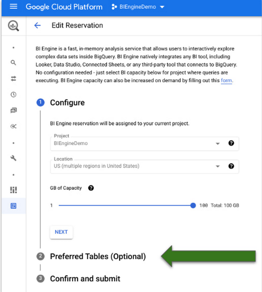
You can simply edit existing BI Engine configuration in the project.  You will see an optional step of specifying the preferred tables, followed by a box to specify the tables you want to set as preferred.

The next step is to confirm and submit the configuration and you will be ready to go! 

Alternatively, you can also achieve this by issuing a DDL statement in SQL editor as follows:

This feature is available in all regions today and rolled out to all BigQuery customers. Please give it a spin!

Editor’s note: Although Twitter has long been considered a treasure trove of data, the task of analyzing Tweets in order to understand what’s happening in the world, what people are talking about right now, and how this information can support business use cases has historically been highly technical and time-consuming. Not anymore. Twitter recently launched an API toolkit for Google Cloud which helps developers to harness insights from Tweets, at scale, within minutes. This blog is based on a conversation with the Twitter team who’ve made this possible. The authors would like to thank Prasanna Selvaraj and Nikki Golding from Twitter for contributions to this blog. 

Businesses and brands consistently monitor Twitter for a variety of reasons: from tracking the latest consumer trends and analyzing competitors, to staying ahead of breaking news and responding to customer service requests. With 229 million monetizable daily active users, it’s no wonder companies, small and large, consider Twitter a treasure trove of data with huge potential to support business intelligence. 

But language is complex, and the journey towards transforming social media conversations into insightful data involves first processing large amounts of Tweets by ways of organizing, sorting, and filtering them. Crucial to this process are Twitter APIs: a set of programmatic endpoints that allow developers to find, retrieve, and engage with real-time public conversations happening on the platform. 

In this blog, we learn from the Twitter Developer Platform Solutions Architecture team about the Twitter API toolkit for Google Cloud, a new framework for quickly ingesting, processing, and analyzing high volumes of Tweets to help developers harness the power of Twitter. 

Making it easier for developers to surface valuable insights from Tweets 

Two versions of the toolkit are currently available: The Twitter API Toolkit for Google Cloud Filtered Stream and the Twitter API Toolkit for Google Cloud Recent Search.

The Twitter API for Google Cloud for Filtered Stream supports developers with a trend detection framework that can be installed on Google Cloud in 60 minutes or less. It automates the data pipeline process to ingest Tweets into Google Cloud, and offers visualization of trends in an easy-to-use dashboard that illustrates real-time trends for configured rules as they unfold on Twitter. This tool can be used to detect macro- and micro-level trends across domains and industry verticals, and can horizontally scale and process millions of Tweets per day. 

“Detecting trends from Twitter requires listening to real-time Twitter APIs and processing Tweets on the fly,” explains Prasanna Selvaraj, Solutions Architect at Twitter and author of this toolkit. “And while trend detection can be complex work, in order to categorize trends, tweet themes and topics must also be identified. This is another complex endeavor as it involves integrating with NER (Named Entity Recognition) and/or NLP (Natural Language Processing) services. This toolkit helps solve these challenges.”

Meanwhile, the Twitter API for Google Cloud Recent Search returns Tweets from the last seven days that match a specific search query. “Anyone with 30 minutes to spare can learn the basics about this Twitter API and, as a side benefit, also learn about Google Cloud Analytics and the foundations of data science,” says Prasanna. 

The toolkits leverage Twitter’s new API v2 (Recent Search & Filtered Stream) and use BigQuery for tweet storage, Data Studio for business intelligence and visualizations, and App Engine for data pipeline on the Google Cloud Platform. 

“We needed a solution that is not only serverless but also can support multi-cardinality, because all Twitter APIs that return Tweets provide data encoded using JavaScript Object Notation (JSON). This has a complex structure, and we needed a database that can easily translate it into its own schema. BigQuery is the perfect solution for this,” says Prasanna. “Once in BigQuery, one can visualize that data in under 10 minutes with Data Studio, be it in a graphic, spreadsheet, or Tableau form. This eliminates friction in Twitter data API consumption and significantly improves the developer experience.” 

Accelerating time to value from 60 hours to 60 minutes

Historically, Twitter API developers have often grappled with processing, analyzing, and visualizing a higher volume of Tweets to derive insights from Twitter data. They’ve had to build data pipelines, select storage solutions, and choose analytics and visualization tools as the first step before they can start validating the value of Twitter data. 

“The whole process of choosing technologies and building data pipelines to look for insights that can support a business use case can take more than 60 hours of a developer’s time,” explains Prasanna. “And after investing that time in setting up the stack they still need to sort through the data to see if what they are looking for actually exists.”

Now, the toolkit enables data processing automation at the click of a button because it provisions the underlying infrastructure it needs to work, such as BigQuery as a database and the compute layer with App Engine. This enables developers to install, configure, and visualize Tweets in a business intelligence tool using Data Studio in less than 60 minutes.

“While we have partners who are very well equipped to connect, consume, store, and analyze data, we also collaborate with developers from organizations who don’t have a myriad of resources to work with. This toolkit is aimed at helping them to rapidly prototype and realize value from Tweets before making a commitment,” explains Nikki Golding, Head of Solutions Architecture at Twitter.

Continuing to build what’s next for developers

As they collaborated with Google Cloud to bring the toolkit to life, the Twitter team started to think about what public datasets exist within the Google Cloud Platform and how they can complement some of the topics that Twitter has a lot of conversations about, from crypto to weather. “We thought, what are some interesting ways developers can access and leverage what both platforms have to offer?” shares Nikki. “Twitter data on its own has high value, but there’s also data that is resident in Google Cloud Platform that can further support users of the toolkit. The combination of Google Cloud Platform infrastructure and application as a service with Twitter’s data as a service is the vision we’re marching towards.”

Next, the Twitter team aims to place these data analytics tools in the hands of any decision-maker, both in technical and non-technical teams. “To help brands visualize, slice, and dice data on their own, we’re looking at self-serve tools that are tailored to the non-technical person to democratize the value of data across organizations,” explains Nikki. “Google Cloud was the platform that allowed us to build the easiest low-code solution relative to others in the market so far, so our aim is to continue collaborating with Google Cloud to eventually launch a no-code solution that helps people to find the content and information they need without depending on developers. Watch this space!”

The MLOps market is expected to grow to around $700m by 20251. With the Google Cloud Professional Data Engineer certification topping the list of highest paying IT certifications in 20212, there has never been a better time to grow your data and ML skills with Google Cloud. 

Introducing the Google Cloud #LearnToEarn challenge 

Starting today, you’re invited to join the data and ML #LearnToEarn challenge– a high-intensity workout for your brain.  Get the ML, data, and AI skills you need to drive speedy transformation in your current and future roles with no-cost access to over 50 hands-on labs on Google Cloud Skills Boost. Race the clock with players around the world, collect badges, and earn special swag! 

How to complete the #LearnToEarn challenge?

The challenge will begin with a core data analyst learning track. Then each week you’ll get new tracks designed to help you explore a variety of career paths and skill sets. Keep an eye out for trivia and flash challenges too!  

As you progress through the challenge and collect badges, you’ll qualify for rewards at each step of your journey. But time and supplies are limited – so join today and complete by July 19! 

What’s involved in the challenge? 

Labs range from introductory to expert level. You’ll get hands-on experience with cutting edge tech like Vertex AI and Looker, plus data differentiators like BigQuery, Tensorflow, integrations with Workspace, and AutoML Vision. The challenge starts with the basics, then gets gradually more complex as you reach each milestone. One lab takes anywhere from ten minutes to about an hour to complete. You do not have to finish all the labs at once – but do keep an eye on start and end dates. 

Ready to take on the challenge?

Join the #LearnToEarn challengetoday!

1. IDC, Market Analysis Perspective: Worldwide AI Life-Cycle Software, September 2021
2. Skillsoft Global Knowledge, 15 top-paying IT certifications list 2021, August 2021

BigQuery BI Engine is a fast, in-memory analysis service that lets users analyze data stored in BigQuery with rapid response times and with high concurrency to accelerate certain BigQuery SQL queries. BI Engine caches data instead of query results, allowing different queries over the same data to be accelerated as you look at different aspects of the data. By using BI Engine with BigQuery streaming, you can perform real-time data analysis over streaming data without sacrificing write speeds or data freshness.

​​BI Engine architecture

The BI Engine SQL interface expands BI Engine support to any business intelligence (BI) tool that works with BigQuery such as Looker, Tableau, Power BI, and custom applications to accelerate data exploration and analysis. With BI Engine, you can build rich, interactive dashboards and reports in BI tool of your choice without compromising performance, scale,security, or data freshness. To learn more about the BI Engine SQL interface, please refer here.

The following diagram shows the updated architecture for BI Engine:

Shown here is one simple example of a Looker dashboard that was created with BI Engine capacity reservation (top) versus the same dashboard without any reservation (bottom).This dashboard is created from the BigQuery public dataset `bigquery-public-data.chicago_taxi_trips.taxi_trips`  to analyze the Sum of total_trip cost and logarithmic average of total trip cost over time.

BI Engine will cache the minimum amount of data possible to resolve a query to maximize the capacity of the reservation. Running business intelligence on big data can be tricky.

Here is a query against the same public dataset, ‘bigquery-public-data.chicago_taxi_trips.taxi_trips,’ to demonstrate BI Engine performance with/without reserved BigQuery slots.

Example Query

The above query was run with the below combinations: 

Without any BigQuery slot reservation/BI Engine reservation,  the query observed 7.6X more average slots and 6.3X more job run time compared to the run with reservations (last stats in the result). 

Without BI Engine reservation but with BigQuery slot reservation, the query observed 6.9X more average slots and 5.9X more job run time compared to the run with reservations (last stats in the result). 

With BI Engine reservation and no BigQuery slot reservation, the query observed 1.5 more average slots and the job completed in sub-seconds (868 ms). 

With both BI Engine reservation and BigQuery slot reservation, only 23 average slots were used and the job completed in sub-second as shown in results.This is the most cost effective way in regards to average slots and run time compared to all other options (23.27 avg_slots , 855 ms run time).

INFORMATION_SCHEMA is a series of views that provide access to metadata about datasets, routines, tables, views, jobs, reservations, and streaming data. You can query the INFORMATION_SCHEMA.JOBS_BY_* view to retrieve real-time metadata about BigQuery jobs. This view contains currently running jobs, and the history of jobs completed in the past 180 days.

Query to determine bi_engine_statistics and number of slots. More schema information can be found here.

From the observation, the most effective way of improving performance  for BI queries is to use BI ENGINE reservation along with BigQuery slot reservation.This will increase query performance, throughput and also utilizes less number of slots. Reserving BI Engine capacity will let you save on slots in your projects.

BigQuery BI Engine optimizes the standard SQL functions and operators when connecting business intelligence (BI) tools to BigQuery. Optimized SQL functions and operators for BI Engine are found here.

Monitor BI Engine with Cloud Monitoring

BigQuery BI Engine integrates with Cloud Monitoring so you can monitor BI Engine metrics and configure alerts.

For information on using Monitoring to create charts for your BI Engine metrics, see Creating charts in the Monitoring documentation.

We ran the same query without BI engine reservation and noticed 15.47 GB were processed.

After BI Engine capacity reservation, in Monitoring under BIE Reservation Used Bytes dashboard we got a compression ratio of ~11.74x (15.47 GB / 1.317 MB). However compression is very data dependent, primarily compression depends on the data cardinality. Customers should run tests on their data to determine their compression rate.

Monitoring metrics ‘Reservation Total Bytes’ gives information about the BI engine capacity reservation whereas ‘Reservation Used Bytes’ gives information about the total used_bytes. Customers can make use of these 2 metrics to come up with the right capacity for reservation. 

When a project has BI engine capacity reserved, queries running in BigQuery will use BI engine to accelerate the compatible subquery performance.​​The degree of acceleration of the query falls into one of the below mentioned modes:

BI Engine Mode FULL – BI Engine compute was used to accelerate leaf stages of the query but the data needed may be in memory or may need to be scanned from a disk. Even when BI Engine compute is utilized, BQ slots may also be used for parts of the query. The more complex the query,the more slots are used.This mode executes all leaf stages in BI Engine (and sometimes all stages).

BI Engine Mode PARTIAL – BI Engine accelerates compatible subqueries and BigQuery processes the subqueries that are not compatible with BI Engine.This mode also provides bi-engine-reason for not using BI Engine mode fully.This mode executes some leaf stages in BI Engine and rest in BigQuery.

BI Engine Mode DISABLED – When BI Engine process subqueries that are not compatible for acceleration, all leaf stages will get processed in BigQuery. This mode also provides bi-engine-reason for not using BI Engine mode fully/partially.

Note that when you purchase a flat rate reservation, BI Engine capacity (GB) will be provided as part of the monthly flat-rate price. You can get up to 100 GB of BI Engine capacity included for free with a 2000-slot annual commitment. As BI Engine reduces the number of slots processed for BI queries, purchasing less slots by topping up little BI Engine capacity along with freely offered capacity might suffice your requirement instead of going in for more slots!

References

bi-engine-introbi-engine-reserve-capacity streaming-apibi-engine-sql-interface-overview bi-engine-pricing bi-engine-sql-interface-overview 

To learn more about how BI Engine and BigQuery can help your enterprise, try out listed Quickstarts page 

bi-engine-data-studiobi-engine-looker Bi-engine-tableau