Archives October 2021

When it comes to anomaly detection, one of the key challenges that many organizations face is that it can be difficult to know how to define what an anomaly is. How do you define and anticipate unusual network intrusions, manufacturing defects, or insurance fraud? If you have labeled data with known anomalies, then you can choose from a variety of supervised machine learning model types that are already supported in BigQuery ML. But what can you do if you don’t know what kind of anomaly to expect, and you don’t have labeled data? Unlike typical predictive techniques that leverage supervised learning, organizations may need to be able to detect anomalies in the absence of labeled data. 

Today we are announcing the public preview of new anomaly detection capabilities in BigQuery ML that leverage unsupervised machine learning to help you detect anomalies without needing labeled data. Depending on whether or not the training data is time series, users can now detect anomalies in training data or on new input data using a new ML.DETECT_ANOMALIES function (documentation), with the following models:

Autoencoder model, now in Public Preview (documentation)

K-means model, already GA (documentation)

ARIMA_PLUS time series model, already GA (documentation)

How does anomaly detection with ML.DETECT_ANOMALIES work?

To detect anomalies in non-time-series data, you can use:

K-means clustering models: When you use ML.DETECT_ANOMALIES with a k-means model, anomalies are identified based on the value of each input data point’s normalized distance to its nearest cluster. If that distance exceeds a threshold determined by the contamination value provided by the user, the data point is identified as an anomaly. 

Autoencoder models: When you use ML.DETECT_ANOMALIES with an autoencoder model, anomalies are identified based on the reconstruction error for each data point. If the error exceeds a threshold determined by the contamination value, it is identified as an anomaly. 

To detect anomalies in time-series data, you can use: 

ARIMA_PLUS time series models: When you use ML.DETECT_ANOMALIES with an ARIMA_PLUS model, anomalies are identified based on the confidence interval for that timestamp. If the probability that the data point at that timestamp occurs outside of the prediction interval exceeds a probability threshold provided by the user, the datapoint is identified as an anomaly.

Below we show code examples of anomaly detection in BigQuery ML for each of the above scenarios.

Anomaly detection with a k-means clustering model

You can now detect anomalies using k-means clustering models, by running ML.DETECT_ANOMALIES to detect anomalies in the training data or in new input data. Begin by creating a k-means clustering model:

With the k-means clustering model trained, you can now run ML.DETECT_ANOMALIES to detect anomalies in the training data or in new input data.

To detect anomalies in the training data, use ML.DETECT_ANOMALIES with the same data used during training:

To detect anomalies in new data, use ML.DETECT_ANOMALIES and provide new data as input:

How does anomaly detection work for k-means clustering models? 

Anomalies are identified based on the value of each input data point’s normalized distance to its nearest cluster, which, if exceeds a threshold determined by the contamination value, is identified as an anomaly. How does this work exactly? With a k-means model and data as inputs, ML.DETECT_ANOMALIES first computes the absolute distance for each input data point to all cluster centroids in the model, then normalizes each distance by the respective cluster radius (which is defined as the standard deviation of the absolute distances of all points in this cluster to the centroid). For each data point, ML.DETECT_ANOMALIES returns the nearest centroid_id based on normalized_distance, as seen in the screenshot above. The contamination value, specified by the user, determines the threshold of whether a data point is considered an anomaly. For example, a contamination value of 0.1 means that the top 10% of descending normalized distance from the training data will be used as the cut-off threshold. If the normalized distance for a datapoint exceeds the threshold, then it is identified as an anomaly. Setting an appropriate contamination will be highly dependent on the requirements of the user or business. 

For more information on anomaly detection with k-means clustering, please see the documentation here.

Anomaly detection with an autoencoder model

You can now detect anomalies using autoencoder models, by running ML.DETECT_ANOMALIES to detect anomalies in the training data or in new input data. 

Begin by creating an autoencoder model:

To detect anomalies in the training data, use ML.DETECT_ANOMALIES with  the same data used during training:

To detect anomalies in new data, use ML.DETECT_ANOMALIES and provide new data as input:

How does anomaly detection work for autoencoder models? 

Anomalies are identified based on the value of each input data point’s reconstructed error, which, if exceeds a threshold determined by the contamination value, is identified as an anomaly. How does this work exactly? With an autoencoder model and data as inputs, ML.DETECT_ANOMALIES first computes the mean_squared_error for each data point between its original values and its reconstructed values. The contamination value, specified by the user, determines the threshold of whether a data point is considered an anomaly. For example, a contamination value of 0.1 means that the top 10% of descending error from the training data will be used as the cut-off threshold. Setting an appropriate contamination will be highly dependent on the requirements of the user or business. 

For more information on anomaly detection with autoencoder models, please see the documentation here.

Anomaly detection with an ARIMA_PLUS time-series model

With ML.DETECT_ANOMALIES, you can now detect anomalies using ARIMA_PLUS time series models in the (historical) training data or in new input data. Here are some examples of when might you want to detect anomalies with time-series data:

Detecting anomalies in historical data: 

Cleaning up data for forecasting and modeling purposes, e.g. preprocessing historical time series before using them to train an ML model.  

When you have a large number of retail demand time series (thousands of products across hundreds of stores or zip codes), you may want to quickly identify which stores and product categories had anomalous sales patterns, and then perform a deeper analysis of why that was the case.

Forward looking anomaly detection: 

Detecting consumer behavior and pricing anomalies as early as possible: e.g. if traffic to a specific product page suddenly and unexpectedly spikes, it might be because of an error in the pricing process that leads to an unusually low price. 

When you have a large number of retail demand time series (thousands of products across hundreds of stores or zip codes), you would like to identify which stores and product categories had anomalous sales patterns based on your forecasts, so you can quickly respond to any unexpected spikes or dips.

How do you detect anomalies using ARIMA_PLUS? Begin by creating an ARIMA_PLUS time series model:

To detect anomalies in the training data, use ML.DETECT_ANOMALIES with the model obtained above:

To detect anomalies in new data, use ML.DETECT_ANOMALIES and provide new data as input:

For more information on anomaly detection with ARIMA_PLUS time series models, please see the documentation here.

Thanks to the BigQuery ML team, especially Abhinav Khushraj, Abhishek Kashyap, Amir Hormati, Jerry Ye, Xi Cheng, Skander Hannachi, Steve Walker, and Stephanie Wang.

A few weeks ago, we launched a new dataset into Google Cloud’s public dataset program: Google Trends. If you’re not familiar with our datasets program, we host a variety of datasets in BigQuery and Cloud Storage for you to access and integrate into your analytics. Google pays for the storage of these datasets and provides public access to the data, e.g., via the bigquery-public-data project. You only pay for queries against the data. Plus, the first 1 TB per month is free! Even better, all of these public datasets will soon be accessible and shareable via Analytics Hub. 

The Google Trends dataset represents the first time we’re adding Google-owned Search data into the program. The Trends data allows users to measure interest in a particular topic or search term across Google Search, from around the United States, down to the city-level. You can learn more about the dataset here, andcheck out the Looker dashboard here! These tables are super valuable in their own right, but when you blend them with other actionable data you can unlock whole new areas of opportunity for your team. You can view and run the queries we demonstrate here.

Focusing on areas that matter

Each day, the top 25 search terms are added to the top_terms table. Additionally, information about how that term has fluctuated over time for each region, Nielsen’s Designated Market Area® (DMA), is recorded with a score. A value of 100 is the peak popularity for the term. This regional information can offer further insight into trends for your organization.

Let’s say I have a BigQuery table that contains information about each one of my physical retail locations. Like we mentioned in our previous blog post, depending on how that data is brought into BigQuery we might enhance the base table by using the Google Maps Geocoding API to convert text-based addresses into lat-lon coordinates.

So now how do I join this data with the Google Trends data? This is where BigQuery GIS functions, plus the public boundaries dataset comes into play. Here I can use the DMA table to determine which DMA each store is in. From there I can simply join back onto the trends data using the DMA ID and focus on the top three terms for each store, which is based on terms with the highest score for that area within the past week. Note that DMA boundaries need to be licensed from Nielsen for use in analysis.

With this information, you can figure out what trends are most important to customers in the areas you care about, which can help you optimize marketing efforts, stock levels, and employee coverage. You may even want to compare across your stores to see how similar term interest is, which may offer new insight into localized product development. 

Filtering for relevant search terms

Search terms are constantly changing and it might not be practical for your team to dig into each and every one.  Instead, you might want to focus your analysis on terms that are relevant to you. Let’s imagine that you have a table that contains all your product names. These names can be long and may contain lots of words or phrases that aren’t necessary for this analysis. For example:

“10oz Authentic Ham and Sausages from Spain”

Like most text problems, you should probably start with some preprocessing. Here, we’re using a simple user-defined functionthat converts the string to lowercase, tokenizes it, and removes words with numbers, and stop words or adjectives that we’ve hard-coded.

For a more robust solution, you might want to leverage a natural language processing package, for example NLTK in Python. You can even process words to use only the stem or find some synonyms to include in your search. Next, you can join the products table onto the trends data, selecting search terms that contain one of the words from the product name.

It looks like `Spain vs Croatia` was recently trending because of the Euro Cup. This might be a great opportunity to create a new campaign and capitalize on momentum: “Spain beat Croatia and is on to the next round, show your support by celebrating with some authentic Spanish ham!” 

Now going a bit further, if we take a look at the top rising search terms from yesterday (as of writing this on 6/30), we can see that there are a lot of names for people.  But it’s unclear who  these people are or why they’re trending. What we do know is we’re looking for a singer to strike up a brand deal with. More specifically, we have a great new jingle for our authentic ham and we’re looking for some trendy singers to bring attention to our company.

Using the Wikipedia Open API you can perform an open search for the term, for example “Jamie Lynn Spears”:

https://en.wikipedia.org/w/api.php?action=opensearch&search=jamie+lynn+spears&limit=1&namespace=0&format=json 

This gives you a JSON response that contains the name of first wikipedia page returned in the search, which you can then use to perform a query against the API:

https://en.wikipedia.org/w/api.php?action=query&prop=extracts&exintro&titles=Jamie_Lynn_Spears&format=json

From here you can grab the first sentence on the page (hint: this usually tells us if the person in question is a singer or not):  “Jamie Lynn Marie Spears (born April 4, 1991) is an American actress and singer.”

Putting this together, we might create a Google Cloud functionthat selects new BigQuery search terms from the table, calls the wikipedia API for each of them, grabs that first sentence and searches for the word “singer.” If we have a hit, then we simply add the search term to the table.Check out some sample code here! Not only does this help us keep track of who the most trendy singers are, but we can use the historical scores to see how their influence has changed over time. 

Staying notified

These queries, plus many more, can be used to make various business decisions. Aside from looking at product names, you might want to keep tabs on competitor names so that you can begin a competitive analysis against rising challengers in your industry. Or maybe you’re interested in a brand deal with a sports player instead of a singer, so you want to make sure you’re aware of any rising stars in the athletic world.  Either way you probably want to be notified when new trends might influence your decision making. 

With another Google Cloud Function, you can programmatically run any interesting SQL queries and return the results in an email. With Cloud Scheduler, you can make sure the function runs each morning, so you stay alert as new trends data is added to the public dataset. Check out the details on how to implement this solution here. 

Ready to get started?

You can explore the new Google Trends dataset in your own project, or if you’re new to BigQuery spin up a project using the BigQuery sandbox. The trends data, along with all the other Google Cloud Public Datasets, will be available in Analytics Hub – so make sure to sign up for the preview, which is scheduled to be available in the third quarter of 2021, by going to g.co/cloud/analytics-hub.

BigQuery is capable of some truly impressive feats, be it scanning billions of rows based on a regular expression, joining large tables, or completing complex ETL tasks with just a SQL query.  One advantage of BigQuery (and SQL in general), is it’s declarative nature. Your SQL indicates your requirements, but the system is responsible for figuring out how to satisfy that request.

However, this approach also has its flaws – namely the problem of understanding intent. SQL represents a conversation between the author and the recipient (BigQuery, in this case). And factors such as fluency and translation can drastically affect how faithfully an author can encode their intent, and how effectively BigQuery can convert the query into a response.

In this week’s BigQuery Admin Reference Guide post, we’ll be providing a more in depth view of query processing. Our hope is that this information will help developers integrating with BigQuery, practitioners looking to optimize queries, and administrators seeking guidance to understand how reservations and slots impact query performance. 

A refresher on architecture

Before we go into an overview of query processing. Let’s revisit BigQuery’s architecture. Last week, we spoke about BigQuery’s native storage on the left hand side. Today, we’ll be focusing on Dremel, BigQuery’s query engine. Note that today we’re talking about BigQuery’s standard execution engine, however BI Engine represents another query execution engine available for fast, in-memory analysis.

As you can see from the diagram, dremel is made up of a cluster of workers.  Each one of these workers executes a part of a task independently and in parallel. BigQuery uses a distributed memory shuffle tier to store intermediate data produced from workers at various stages of execution. The shuffle leverages some fairly interesting Google technologies, such as our very fast petabit network technology, and RAM wherever possible. Each shuffled row can be consumed by workers as soon as it’s created by the producers.

This makes it possible to execute distributed operations in a pipeline. Additionally, if a worker has partially written some of its output and then terminated (for example, the underlying hardware suffered a power event), that unit of work can simply be re-queued and sent to another worker.  A failure of a single worker in a stage doesn’t mean all the workers need to re-run. 

When a query is complete, the results are written out to persistent storage and returned to the user. This also enables us to serve up cached results the next time that query executes. 

Overview of query processing

Now that you understand the query processing architecture, we’ll run through query execution at a high level, to see how each step comes together.  

First Steps: API request management

BigQuery supports an asynchronous API for executing queries: callers can insert a query job request, and then poll it until complete –as we discussed a few weeks ago.  BigQuery supports a REST-based protocol for this, which accepts queries encoded via JSON.

To proceed, there’s some level of API processing that must occur.  Some of things that must be done are authenticating and authorizing the request, plus building and tracking associated metadata such as the SQL statement, cloud project, and/or query parameters.

Decoding the query text: Lexing and parsing

Lexing and parsing is a common task for programming languages, and SQL is no different.  Lexing refers to the process of scanning an array of bytes (the raw SQL statement) and converting that into a series of tokens. Parsing is the process of consuming those tokens to build up a syntactical representation of the query that can be validated and understood by BigQuery’s software architecture.

If you’re super interested in this, we recommend checking out the ZetaSQL project, which includes the open source reference implementation of the SQL engine used by BigQuery and other GCP projects.

Referencing resources: Catalog resolution

SQL commonly contains references to entities retained by the BigQuery system – such as tables, views, stored procedures and functions. For BigQuery to process these references, it must resolve them into something more comprehensible.  This stage helps the query processing system answer questions like:

Is this a valid identifier?  What does it reference?

Is this entity a managed table, or a logical view?

What’s the SQL definition for this logical view?

What columns and data types are present in this table?

How do I read the data present in the table?  Is there a set of URIs I should consume?

Resolutions are often interleaved through the parsing and planning phases of query execution.

Building a blueprint: Query planning

As a more fully-formed picture of the request is exposed via parsing and resolution, a query plan begins to emerge.  Many techniques exist to refactor and improve a query plan to make it faster and more efficient.  Algebraization, for example, converts the parse tree into a form that makes it possible to refactor and simplify subqueries.  Other techniques can be used to optimize things further,  moving tasks like pruning data closer to data reads (reducing the overall work of the system).

Another element is adapting it to run as a set of distributed execution tasks.  Like we mentioned in the beginning of this post, BigQuery leverages large pools of query computation nodes, or workers. So, it must coordinate how different stages of the query plan share data through reading and writing from storage, and how to stage temporary data within the shuffle system.

Doing the work: Query execution

Query execution is simply the process of working through the query stages in the execution graph, towards completion.  A query stage may have a single unit of work, or it may be represented by many thousands of units of work, like when a query stage reads all the data in a large table composed of many separate columnar input files.

Query management: scheduling and dynamic planning

Besides the workers that perform the work of the query plan itself, additional workers monitor and direct the overall progress of work throughout the system. Scheduling is concerned with how aggressively work is queued, executed and completed.

However, an interesting property of the BigQuery query engine is that it has dynamic planning capabilities.  A query plan often contains ambiguities, and as a query progresses it may need further adjustment to ensure success.  Repartitioning data as it flows through the system is one example of a plan adaptation that may be added, as it helps ensure that data is properly balanced and sized for subsequent stages to consume.

Finishing up: finalizing results

As a query completes, it often yields output artifacts in the form of results, or changes to tables within the system.  Finalizing results includes the work to commit these changes back to the storage layer. BigQuery also needs to communicate back to you, the user, that the system is done processing the query. The metadata around the query is updated to note the work is done, or the error stream is attached to indicate where things went wrong.

Understanding query execution

Armed with our new understanding of the life of a query, we can dive more deeply into query plans.  First, let’s look at a simple plan. Here, we are running a query against a public BigQuery dataset to count the total number of citi bike trips that began at stations with “Broadway” in the name. 

SELECT COUNT(*)

FROM `bigquery-public-data.new_york.citibike_trips`

WHERE start_station_name LIKE “%Broadway%”

Now let’s consider what is happening behind the scenes when BigQuery processes this query. 

First, a set of workers access the distributed storage to read the table, filter the data, and generate partial counts. Next, these workers send their counts to the shuffle.

The second stage reads from those shuffle records as its input, and sums them together. It then writes the output file into a single file, which becomes accessible as the result of the query.

You can clearly see that the workers don’t communicate directly with one another at all; they communicate through reading and writing data. After running the query in the BigQuery console, you can see the execution details and gather information about the query plan (note that the execution details shown below may be slightly different than what you see in the console since this data changes). 

Note that you can also get execution details from the information_schema tables or the Jobs API. For example, by running:

SELECT

*

FROM

`region-us`.INFORMATION_SCHEMA.JOBS_BY_PROJECT

WHERE

job_id = “bquxjob_49c5bc47_17ad3d7778f”

Interpreting the query statistics

Query statistics include information about how many work units existed in a stage, as well as how many were completed.  For example, inspecting the result of the information schema query used earlier we can get the following:

Input and output

Using the parallel_inputs field, we can see how finely divided the input is. In the case of a table read, it indicates how many distinct file blocks were in the input.  In the case of a stage that reads from shuffle, the number of inputs tells us how many distinct data buckets are present.  Each of these represent a distinct unit of work that can be scheduled independently. So, in our case, there are 57 different columnar file blocks in the table. 

In this representation, we can also see the query scanned more than 33 million rows while processing the table.  The second stage read 57 rows, as the shuffle system contained one row for each input from the first stage. 

It’s also perfectly valid for a stage to finish with only a subset of the inputs processed.  Cases where this happens tend to be execution stages where not all the inputs need to be processed to satisfy what output is needed; a common example of this might be a query stage that consumes part of the input and uses a LIMIT clause to restrict the output to some smaller number of rows.

It is also worth exploring the notion of parallelism.  Having 57 inputs for a stage doesn’t mean the stage won’t start until there’s 57 workers (slots) available.  It means that there’s a queue of work with 57 elements to work through.  You can process that queue with a single worker, in which case you’ve essentially got a serial execution.  If you have multiple workers, you can process it faster as they’re working independently to process the units.  However, more than 57 slots doesn’t do anything for you; the work cannot be more finely distributed.

Aside from reading from native distributed storage, and from shuffle, it’s also possible for BigQuery to perform data reads and writes from external sources, such as Cloud Storage (as we discussed in our earlier post). In such cases the notion of parallel access still applies, but it’s typically less performant. 

Slot utilization

BigQuery communicates resource usage through a computational unit known as a slot. It’s simplest to think of it as similar to a virtual CPU and it’s a measure that represents the number of workers available / used. When we talk about slots, we’re talking about overall computational throughput, or rate of change.  For example, a single slot gives you the ability to make 1 slot-second of compute progress per second.  As we just mentioned, having fewer workers – or less slots – doesn’t mean that a job won’t run. It simply means that it may run slower. 

In the query statistics, we can see the amount of slot_ms (slot-milliseconds) consumed. If we divide this number by the amount of milliseconds it took for the query stage to execute, we can calculate how many fully saturated slots this stage represents. 

SELECT job_stages.name, job_stages.slot_ms/(job_stages.end_ms – job_stages.start_ms) as full_slots

FROM

`region-us`.INFORMATION_SCHEMA.JOBS_BY_PROJECT

, UNNEST(job_stages) as job_stages

WHERE

job_id = “bquxjob_49c5bc47_17ad3d7778f”

This information is helpful, as it gives us a view of how many slots are being used on average across different workloads or projects – which can be helpful for sizing reservations (more on that soon). If you see areas where there is a higher number of parallel inputs compared to fully saturated slots, that may represent a query that will run faster if it had access to more slots. 

Time spent in phases

We can also see the average and maximum time each of the workers spent in the wait, read, compute and write phase for each stage of the query execution:

Wait Phase: the engine is waiting for either workers to become available or for a previous stage to start writing results that it can begin consuming. A lot of time spent in the wait phase may indicate that more slots would result in faster processing time. 

Read Phase: the slot is reading data either from distributed storage or from shuffle.  A lot of time spent here indicates that there might be an opportunity to limit the amount of data consumed by the query (by limiting the result set or filtering data). 

Compute Phase: where the actual processing takes place, such as evaluating SQL functions or expressions. A well-tuned query typically spends most of its time in the compute phase. Some ways to try and reduce time spent in the compute phase are to leverage approximation functions or investigate costly string manipulations like complex regexes. 

Write phase: where data is written, either to the next stage, shuffle, or final output returned to the user. A lot of time spent here indicates that there might be an opportunity to limit the results of the stage (by limiting the result set or filtering data)

If you notice that the maximum time spent in each phase is much greater than the average time, there may be an uneven distribution of data coming out of the previous stage. One way to try and reduce data skew is by filtering early in the query.

Large shuffles

While many query patterns use reasonable volumes of shuffle, large queries may exhaust available shuffle resources. Particularly, if you see that a query stage is heavily attributing its time spent to writing out to shuffle, take a look at the shuffle statistics.  The shuffleOutputBytesSpilled tells us if the shuffle was forced to leverage disk resources beyond in-memory resources. 

SELECT job_stages.name, job_stages.shuffle_output_bytes_spilled

FROM

`region-us`.INFORMATION_SCHEMA.JOBS_BY_PROJECT

, UNNEST(job_stages) as job_stages

WHERE

job_id = “bquxjob_49c5bc47_17ad3d7778f”

Note that a disk-based write takes longer than an in-memory write. To prevent this from happening, you’ll want to filter or limit the data so that less information is passed to the shuffle. 

Tune in next week

Next week, we’ll be digging into more advanced queries and talking through tactical query optimization techniques so make sure to tune in! You can keep an eye out for more in this series by following Leigha on LinkedIn and Twitter.

Editor’s note: Today we’re hearing from Sagar Batchu, Director of Engineering at LiveRamp. He shares how Google Cloud helped LiveRamp modernize its data analytics infrastructure to simplify its operations, lower support and infrastructure costs and enable its customers to connect, control, and activate customer data safely and securely. 

LiveRamp is a data connectivity platform that provides best in class identity resolution, activation and measurement for customer data so businesses can create a true customer 360 degree view. We run data engineering workloads at scale, often processing petabytes of customer data every day via LiveRamp Connect platform APIs. 

As we integrated more internal and external APIs and the sophistication of our product offering grew, the complexity of our data pipelines increased. The status quo for building data pipelines very quickly became painful and cumbersome as these processes take time and knowledge of an increasingly complex data engineering stack. Pipelines became harder to maintain as the dependencies grew and the codebase became increasingly unruly.

Beginning last year, we set out to improve these processes and re-envision how we reduce time to value for data teams by thinking of our canonical ETL/LT analytics pipelines as a set of reusable components. We wanted teams to spend their time adding new features which encapsulate business value rather than spending time figuring out how to run workloads at scale on cloud infrastructure. This was even more pertinent with data science, data analyst and services teams whose daily wheelhouse was not the nitty gritty of deploying pipelines. 

With all this in mind, we decided to start a data operations initiative, a concept popularised in the last few years, which aims to accelerate the time to value for data-oriented teams by allowing different personas in the data engineering lifecycle to focus on the “what” rather than the “how.”  

We chose Google Cloud to execute on this initiative to speed up our transformation. Our architectural optimizations, coupled with Google Cloud’s platform capabilities simplified our operational model, reduced time to value, and greatly improved the portability of our data ecosystem for easy collaboration. Today, we have ten teams across LiveRamp running hundreds of workloads a day, and in the next quarter, we plan to scale to thousands. 

Why LiveRamp Chose Google Cloud 

Google Cloud provides all the necessary services in a serverless fashion to build complex data applications and run massive infrastructure. Google Cloud offers data analytics capabilities that help organizations like LiveRamp to easily capture, manage, process and visualize data at scale. Many of the Google Cloud data processing platforms also have open source roots making them extremely collaborative. One such platform is CDAP (Cask Data Application Platform), which Cloud Data Fusion is built on. We were drawn to this for the following reasons:

CDAP is inherently multicloud. Pipeline building blocks known as Plugins define individual units of work. They can be run through different provisioners which implement managed cloud runtimes.

The control plane is a set of microservices hosted on Kubernetes, whereas the data plane leverages the best of breed big data cloud products such as Dataproc.

It is built as a framework and is inherently extensible, and decoupled from the underlying architecture. We can extend it both at the system and user-level through “extensions” and “plugins” respectively. For example, we were able to add a system extension for LiveRamp specific authorisation and build a plugin that encompasses common LiveRamp identity operations.

It is open sourced, and there is a dedicated team at Google Cloud building and maintaining the core codebase as well as a growing suite of source, transform and sink connectors.

It aligns with ourremote execution and non-data movement strategy. CDAP executes pipelines remotely and manages through a stream of metadata via public cloud APIs. 

CDAP supports an SRE mindset by providing out of the box monitoring and observability tooling.

It has a rich set of APIs backed by scalable microservices to provide ETL as a Service to other teams.

Cloud Data Fusion, Google Cloud’s fully managed, native data integration platform is based on CDAP. We benefit from the managed security features of Data Fusion like IAM integration, customer manager encryption keys, role based access controls and data residency to ensure stricter governance requirements around data isolation. 

How are teams using the Data Operations Platform? 

Through this initiative, we have encouraged data science and engineering teams to focus on business logic and leave data integrations and infrastructure as separate concerns. A centralised team runs CDAP as a service, and custom plugins are hosted in a democratized plugin marketplace where any team can contribute their canonical operations.

Adoption of the platform was driven by one of our most common patterns of data pipelining: The need to resolve customer data using our Identity APIs. LiveRamp Identity APIs connect fragmented and inaccurate customer identity by providing a way to resolve PII to pseudonymous identifiers. This enables client brands to connect, control, and activate customer data safely and securely. 

The reality of customer data is that it lives in a variety of formats, storage locations, and often needs bespoke cleanup. Before, technical services teams at LiveRamp had to develop expensive processes to manage these hygiene and validation processes even before the data was resolved to an identity. Over time, a combination of bash and python scripts and custom ETL pipelines became untenable. 

By implementing our most used Identity APIs, a series of CDAP plugins, our customers were able to operationalise their processes by logging into a Low Code user interface, select a source of data, run standard validation and hygiene steps, visually inspect using CDAP’s Wrangler interface for especially noisy cases, and channel data into our Identity API. As these workflows became validated, they have been established as standard CDAP pipelines that can now be parameterized and distributed on the internal marketplace. These technical services teams have not only reduced their time to value but have also enabled future teams to leverage their customer pipelines without worrying about the portability to other team’s infrastructures.

What’s Next ? 

With critical customer use cases now powered by CDAP, we plan on scaling out usage of the platform to the next batch of teams. We plan on taking on more complex pipelines, cross-team workloads, and adding support for the ever growing LiveRamp platform API suite.

In addition to the Google Cloud community and the external community, we have a growing base of LiveRamp developers building out plugins on CDAP to support routine transforms and APIs. These are used by other teams who push the limits and provide feedback — spinning a flywheel of collaboration between those who build and those who operate. Furthermore, teams internally can continue to use their other favorite data tools like BigQuery and Airflow as we continue to deeply integrate CDAP into our internal data engineering ecosystem. 

Our data operations platform powered by CDAP is quickly becoming a center point for data teams – a place to ingest, hygiene, transform, and sink their data consistently.

We are excited by Google Cloud’s roadmap for CDAP and Data Fusion. Support for new execution engines, data sources and sinks, and new features like Datastream and Replication will mean LiveRamp teams can continue to trust that their applications will be able to interoperate with the ever evolving cloud data engineering ecosystem.

Our goal is to continue to improve our platform functionalities, and find new ways to empower Looker developers to build data experiences much faster and at a lower upfront cost.

We’ve heard the developer community feedback and we’re excited to have announced the general availability of the Looker Extension Framework.

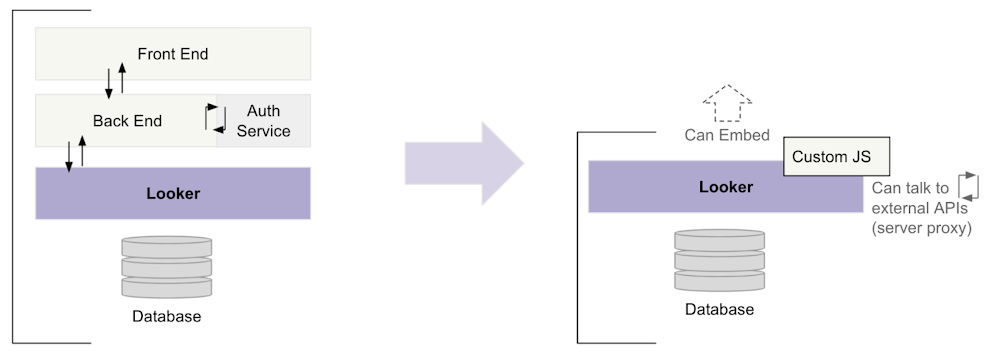
The Extension Framework is a fully hosted development platform that enables developers to build any data-powered application, workflow or tool right in Looker. By eliminating the need to spin up and host infrastructure, the Extension Framework lets developers focus on building great experiences for their users. Traditionally, customers and partners who build custom applications with Looker, have to assemble an entire development infrastructure before they can proceed with implementation. For instance, they might need to stand up both a back end and front end and then implement services for hosting and authorization. This leads to additional time and cost spent.

The Extension Framework eliminates all development inefficiency and helps significantly reduce friction in the setup and  development process, so developers can focus on starting development right away. Looker developers would no longer need DevOps or infrastructure to host their data applications and these applications (when built on the Extension Framework), can take full advantage of the power of Looker. To enable these efficiencies, the Looker Extension Framework includes a streamlined way to leverage the Looker APIs and SDKs, UI components for building the visual experience, as well as authentication, permission management and application access control. 

Content created via the Extension Framework can be built as a full-screen experience or embedded into an external website or application. We will soon be adding functionality to allow  for the embedding of extensions inside Looker (as a custom tile you plug into your dashboard, for example). Through our Public Preview period we have already seen over 150+ extensions deployed to production users, with an additional 200+ extensions currently in development. These extensions include solutions like: enhanced navigation tools, customized navigation and modified reporting applications, to name a few.

Extension Framework Feature Breakdown

The Looker Extension Framework includes the following features:

The Looker Extension SDK, which provides functions for Looker public API access and for interacting within the Looker environment.

Looker components, a library of pre-built React UI components you can use in your extensions.

The Embed SDK, a library you can use to embed dashboards, Looks, and Explores in your extension. 

The create-looker-extension utility, an extension starter kit that includes all the necessary extension files and dependencies.

Our Looker extension framework examples repo, with templates and sample extensions to assist you in getting started quickly.

The ability to access third-party API endpoints and add third-party data to your extension in building enhanced data experiences (e.g. Google Maps API).

The ability to create full-screen extensions within Looker. Full-screen extensions can be used for internal or external platform applications.

The ability to configure an access key for your extension so that users must enter a key to run the extension. 

Next Steps

If you haven’t yet tried the Looker Extension Framework, we think you’ll find it to be a major upgrade to your data app development experience. Over the next few months, we will continue to make enhancements to the Extension Framework with the goal of significantly reducing the amount of code required, and eventually empowering our developers with a low-code, no-code framework.

Comprehensive details and examples that help you get started in developing with the Extension Framework are now available here. We hope that these new capabilities inspire your creativity and we’re super excited to see what you build with the Extension Framework!

With data volumes constantly growing, many companies find it difficult to use data effectively and gain insights from it. Often these organizations are burdened with cumbersome and difficult-to-maintain data architectures. 

One way that companies are addressing this challenge is with change streaming: the movement of data changes as they happen from a source (typically a database) to a destination. Powered by change data capture (CDC), change streaming has become a critical data architecture building block. We recently announced Datastream, a serverless change data capture and replication service. Datastream’s key capabilities include:

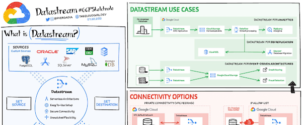
Replicate and synchronize data across your organization with minimal latency. You can synchronize data across heterogeneous databases and applications reliably, with low latency, and with minimal impact to the performance of your source. Unlock the power of data streams for analytics, database replication, cloud migration, and event-driven architectures across hybrid environments.Scale up or down with a serverless architecture seamlessly. Get up and running fast with a serverless and easy-to-use service that scales seamlessly as your data volumes shift. Focus on deriving up-to-date insights from your data and responding to high-priority issues, instead of managing infrastructure, performance tuning, or resource provisioning.Integrate with the Google Cloud data integration suite. Connect data across your organization with Google Cloud data integration  products. Datastream leverages Dataflow templates to load data into BigQuery, Cloud Spanner, and Cloud SQL; it also powers Cloud Data Fusion’s CDC Replicator connectors for easier-than-ever data pipelining.

Datastream use cases

Datastream captures change streams from Oracle, MySQL, and other sources for destinations such as Cloud Storage, Pub/Sub, BigQuery, Spanner and more. Some use cases of Datastream:  

For analytics use Datastream with a pre-built Dataflow template to create up-to-date replicated tables in BigQuery in a fully-managed way.For database replication use Datastream with pre-built Dataflow templates to continuously replicate and synchronize database data into Cloud SQL for PostgreSQL or Spanner to power low-downtime database migration or hybrid-cloud configuration.For building event-driven architectures use Datastream to ingest changes from multiple sources into object stores like Google Cloud Storage or, in the future, messaging services such as Pub/Sub or Kafka Streamline real-time data pipeline that continually streams data from legacy relational data stores (like Oracle and MySQL) using Datastream into MongoDB. 

How do you set up Datastream?

Create a source connection profile.Create a destination connection profile.Create a stream using the source and destination connection profiles, and define the objects to pull from the source.Validate and start the stream.

Once started, a stream continuously streams data from the source to the destination. You can pause and then resume the stream. 

Connectivity options

To use Datastream to create a stream from the source database to the destination, you must establish connectivity to the source database. Datastream supports the IP allowlist, forward SSH tunnel, and VPC peering network connectivity methods.

Private connectivity configurations enable Datastream to communicate with a data source over a private network (internally within Google Cloud, or with external sources connected over VPN or Interconnect). This communication happens through a Virtual Private Cloud (VPC) peering connection. 

For a more in-depth look into Datastream check out the documentation.

For more #GCPSketchnote, follow the GitHub repo. For similar cloud content follow me on Twitter @pvergadia and keep an eye out on thecloudgirl.dev.

As the Olympics kicked off in Tokyo at the end of July, we found ourselves reflecting on the beauty of diverse countries and cultures coming together to celebrate greatness and sportsmanship. For this month’s blog, we’d like to highlight some key data and analytics performances that should help inspire you to reach new heights in your data journey.

Let’s review the highlights!

BigQuery ML Anomaly Detection: A perfect 10 for augmented analytics

Identifying anomalous behavior at scale is a critical component of any analytics strategy. Whether you want to work with a single frame of data or a time series progression, BigQuery ML allows you to bring the power of machine learning to your data warehouse. 

In this blog released at the beginning of last month, our team walked through both non-time series and time-series approaches to anomaly detection in BigQuery ML:

Non-time series anomaly detection

Autoencoder model (now in Public Preview)

K-means model (already in GA)

Time-series anomaly detection

ARIMA_PLUS time series model (already in GA)

These approaches make it easy for your team to quickly experiment with data stored in BigQuery to identify what works best for your particular anomaly detection needs. Once a model has been identified as the right fit, you can easily port that model into the Vertex AI platform for real-time analysis or schedule it in BigQuery for continued batch processing.

App Analytics: Winning the team event

Google provides a broad ecosystem of technologies and services aimed at solving modern day challenges. Some of the best solutions come when those technologies are combined with our data analytics offerings to surface additional insights and provide new opportunities. 

Firebase has deep adoption in the app development community and provides the technology backbone for many organization’s app strategy. This month we launched a design pattern that shows Firebase customers how to use Crashlytics data, CRM, issue tracking, and support data in BigQuery and Looker to identify opportunities to improve app quality and enhance customer experiences.

Crux on BigQuery: Taking gold in the all-around data competition

Crux Informatics provides data services to many large companies to help their customers make smarter business decisions. While they were already operating on a modern stack and not on the hunt for a modern data warehouse, BigQuery became an enticing option due to performance and a more optimal pricing model. Crux also found advantages with lower-cost ingestion and processing engines like Dataflow that allow for streaming analytics.

Technology is a team sport, and Crux found our support team responsive and ready to help. This decision to more deeply adopt Google Cloud’s data analytics offerings provides Crux with the flexibility to manage a constantly evolving data ecosystem and stay competitive.

You can read more about Crux’s decision to adopt BigQuery in this blog.

Google Trends: A classic emerges a champion

Following up on the launch of our Google Trends dataset in June, we delivered some examples of how to use that data to augment your decision making. 

As a quick recap of that dataset, Google Cloud, and in particular BigQuery, provide access to the top 25 trending terms by Nielsen’s Designated Market Area® (DMA) with a weekly granularity. These trending terms are based on search patterns and have historically only been available on the Google Trends website.

The Google Trends design pattern addresses some common business needs, such as identifying what’s trending geographically near your stores and how to match trending terms to products to identify potential campaigns. 

Dataflow GPU: More power than ever for those streaming sprints

Dataflow is our fully-managed data processing platform that supports both batch and streaming workloads. The ability of Dataflow to scale and easily manage unbounded data has made it the streaming solution of choice for large workloads with high-speed needs in Google Cloud. 

But what if we could take that speed and provide even more processing power for advanced use cases? Our team, in partnership with NVIDIA, did just that by adding GPU support to Dataflow. This allows our customers to easily accelerate compute-intensive processing like image analysis and predictive forecasting with amazing increases in efficiency and speed. 

Take a look at the times below:

Data Fusion: A play-by-play for data integration’s winning performance

Data Fusion provides Google Cloud customers with a single place to perform all kinds of data integration activities. Whether it’s ETL, ELT, or simply integrating with a cloud application, Data Fusion provides a clean UI and streamlined experience with deep integrations to other Google Cloud data systems. Check out our team’s review of this tool and the capabilities it can bring to your organization.

Google provides a set of Dataflow templates that customers commonly use for frequent data tasks, but also as reference data pipelines that developers can extend. But what if you want to customize a Dataflow template without modifying or maintaining the Dataflow template code itself? With user-defined functions (UDFs), customers can extend certain Dataflow templates with their custom logic to transform records on the fly:

A UDF is a JavaScript snippet that implements a simple element processing logic, and is provided as an input parameter to the Dataflow pipeline. This is especially helpful for users who want to customize the pipeline’s output format without having to re-compile or to maintain the template code itself. Example use cases include enriching records with additional fields, redacting some sensitive fields, or filtering out undesired records – we’ll dive into each of those. That means you do not have to be an Apache Beam developer or even have a developer environment setup in order to tweak the output of these Dataflow templates!

At the time of writing, the following Google-provided Dataflow templates support UDF:

Pub/Sub to BigQuery

Pub/Sub to Datastore

Pub/Sub to Splunk

Pub/Sub to MongoDB

Datastore to GCS Text

Datastore to Pub/Sub

Cloud Spanner to Cloud Storage Text

GCS Text to Datastore

GCS Text to BigQuery (Batch and Stream)

Apache Kafka to BigQuery

Datastore Bulk Delete

Note: While the UDF concepts described here apply to any Dataflow template that supports UDF, the utility UDF samples below are from real-world use cases using the Pub/Sub to Splunk Dataflow template, but you can re-use those as starting point for this or other Dataflow templates. 

How UDF works with templates

When a UDF is provided, the UDF JavaScript code runs on Nashorn JavaScript engine included in the Dataflow worker’s Java runtime (applicable for Java pipelines such as Google-provided Dataflow templates). The code is invoked locally by a Dataflow worker for each element separately. Element payloads are serialized and passed as JSON strings back and forth.

Here’s the format of a Dataflow UDF function called process which you can reuse and insert your own custom transformation logic into:

Using JavaScript’s standard built-in JSON object, the UDF first parses the stringified element inJson into a variable obj, and, at the end, it must return a stringified version outJson of the modified element obj. Where highlighted, you add your custom element transformation logic depending on your use case. In the next section, we provide you with utility UDF samples from real-world use cases. 

Note: The variable includePubsubMessage is required if the UDF is applied to Pub/Sub to Splunk Dataflow template since it supports two possible element formats: that specific template can be configured to process the full Pub/Sub message payload or only the underlying Pub/Sub message data payload (default behavior). The statement setting data variable is needed to normalize the UDF input payload in order to simplify your subsequent transformation logic in the UDF, consistent with the examples below. For more context, see includePubsubMessage parameter in Pub/Sub to Splunk template documentation.

Common UDF patterns

The following code snippets are example transformation logic to be inserted in the above UDF process function. They are grouped below by common patterns.

Pattern 1: Enrich events

Follow this pattern to enrich events with new fields for more contextual information.

Example 1.1:

Add a new field as metadata to track pipeline’s input Pub/Sub subscription

Example 1.2*:

Set Splunk HEC metadata source field to track pipeline’s input Pub/Sub subscription

Add new fields based on a user-defined local function e.g. callerToAppIdLookup() acting as a static mapping or lookup table

Pattern 2: Transform events

Follow this pattern to transform the entire event format depending on what your destination expects.

Revert logs from Cloud Logging log payload (LogEntry) to original raw log string. You may use this pattern with VM application or system logs (e.g. syslog or Windows Event Logs) to send source raw logs (instead of JSON payloads):

Transform logs from Cloud Logging log payload (LogEntry) to original raw log string by setting Splunk HEC event metadata. Use this pattern with application or VM logs (e.g. syslog or Windows Event Logs) to index original raw logs (instead of JSON payload) for compatibility with downstream analytics. This example also enriches logs by setting HEC fields metadata to incoming resource labels metadata:

Pattern 3: Redact events

Follow this pattern to redact or remove a part of the event.

Delete or redact sensitive SQL query field from BigQuery AuditData data access logs:

Pattern 4: Route events

Follow this pattern to programmatically route events to separate destinations.

Example 4.1*:

Route event to the correct Splunk index per used-defined local function e.g. splunkIndexLookup() acting as a static mapping or lookup table:

Route unrecognized or unsupported events to Pub/Sub deadletter topic (if configured) in order to avoid invalid data or unnecessary consumption of downstream sinks such as BigQuery or Splunk:

Pattern 5: Filter events

Follow this pattern to filter out undesired or unrecognized events.

Example 5.1:

Drop events from a particular resource type or log type, e.g. filter out verbose Dataflow operational logs such as worker & system logs:

Drop events from a particular log type, e.g. Cloud Run application stdout:

* Example applicable to Pub/Sub to Splunk Dataflow template only

Testing UDFs

Besides ensuring functional correctness, you must verify your UDF code is syntactically correct JavaScript on Oracle Nashorn JavaScript engine which is shipped as part of JDK (8 through 14) pre-installed in Dataflow workers. That’s where your UDF ultimately runs. Before pipeline deployment, it is highly recommended to test your UDF on Nashorn engine: any JavaScript syntax error will throw an exception, potentially on every message. This will cause a pipeline outage as the UDF is unable to process those messages in-flight.

At the time of this writing, Google-provided Dataflow templates run on JDK 11 environment with the corresponding Nashorn engine v11 release. By default, Nashorn engine is only ECMAScript 5.1 (ES5) compliant so a lot of newer ES6 JavaScript keywords like let or const will cause syntax errors. In addition, it’s important to note that Nashorn engine is a slightly different JavaScript implementation than Node.js. A common pitfall is using console.log() or Number.isNaN() for example, neither of which are defined in the Nashorn engine. For more details, see this introduction to using Oracle Nashorn. That said, using the utility UDFs provided above without major code changes should be sufficient for most use cases.

An easy way to test your UDF on Nashorn engine is by launching Cloud Shell where JDK 11 is pre-installed, including jjs command-line tool to invoke Nashorn engine.

Let’s assume your UDF is saved in dataflow_udf_transform.js JavaScript file and that you’re using UDF example 1.1 above which appends new inputSubscription field.

In Cloud Shell, you can launch Nashorn in interactive mode as follows:

In Nashorn interactive shell, first load your UDF JavaScript file which will load the UDF ‘process’ function in global scope:

To test your UDF, define an arbitrary input JSON object depending on your pipeline’s expected in-flight messages. In this example, we’re using a snippet of a Dataflow job log message to be processed by our pipeline:

You can now invoke your UDF function to process that input object as follows:

Notice how the input object is serialized first before being passed to UDF which expects an input string as noted in the previous section.

Print the UDF output to view the transformed log with the appended inputSubscription field as expected:

Finally exit the interactive shell:

Deploying UDFs

You deploy a UDF when you run a Dataflow job by referencing a GCS file containing the UDF JavaScript file. Here’s an example using gcloud CLI to run a job using the Pub/Sub to Splunk Dataflow template:

The relevant parameters to configure:

gcs-location: GCS location path to the Dataflow template

javascriptTextTransformGcsPath: GCS location path to JavaScript file with your UDF code

javascriptTextTransformFunctionName: Name of JavaScript function to call as your UDF

As a Dataflow user or operator, you simply reference a pre-existing template URL (Google-hosted), and your custom UDF (Customer-hosted) without the requirement to have a Beam developer environment setup or to maintain the template code itself.

Note: The Dataflow worker service account used must have access to the GCS object (JavaScript file) containing your UDF function. Refer to Dataflow user docs to learn more about Dataflow worker service account.

What’s Next?

We hope this helps you get started with customizing some of the off-the-shelf Google-provided Dataflow templates using one of the above utility UDFs or writing your own UDF function. As a technical artifact of your pipeline deployment, the UDF is a component of your infrastructure, and so we recommend you follow Infrastructure-as-Code (IaC) best practices including version-controlling your UDF. If you have questions or suggestions for other utility UDFs, we’d like to hear from you: create an issue directly in GitHub repo, or ask away in our Stack Overflow forum.

In a follow-up blog post, we’ll dive deeper into testing UDFs (unit tests and end-to-end pipeline tests) as well as setting up a CI/CD pipeline (for your pipelines!) including triggering new deployment every time you update your UDFs – all without maintaining any Apache Beam code.